Sloan Digital Sky Survey: Early Data Release
Chris Stoughton, Robert H. Lupton, Mariangela Bernardi, Michael R. Blanton, Scott Burles, Francisco J. Castander, A. J. Connolly, Daniel J. Eisenstein, Joshua A. Frieman, G. S. Hennessy, Robert B. Hindsley, Zeljko Ivezi\'c, Stephen Kent, Peter Z. Kunszt, Brian C. Lee, Avery Meiksin, Jeffrey A. Munn, Heidi Jo Newberg, R. C. Nichol, Tom Nicinski, Jeffrey R. Pier, Gordon T. Richards, Michael W. Richmond, David J. Schlegel, J. Allyn Smith, Michael A. Strauss, Mark SubbaRao, Alexander S. Szalay, Aniruddha R. Thakar, Douglas L. Tucker, Daniel E. Vanden Berk, Brian Yanny, Jennifer K. Adelman, John E. Anderson, Jr., Scott F. Anderson, James Annis, Neta A. Bahcall, J. A. Bakken, Matthias Bartelmann, Steven Bastian, Amanda Bauer, Eileen Berman, Hans Böhringer, William N. Boroski, Steve Bracker, Charlie Briegel, John W. Briggs, J. Brinkmann, Robert Brunner, Larry Carey, Michael A. Carr, Bing Chen, Damian Christian, Patrick L. Colestock, J. H. Crocker, István Csabai, Paul C. Czarapata, Julianne Dalcanton, Arthur F. Davidsen, John Eric Davis, Walter Dehnen, Scott Dodelson, Mamoru Doi, Tom Dombeck, Megan Donahue, Nancy Ellman, Brian R. Elms, Michael L. Evans, Laurent Eyer, Xiaohui Fan, Glenn R. Federwitz, Scott Friedman, Masataka Fukugita, Roy Gal, Bruce Gillespie, Karl Glazebrook, Jim Gray, Eva K. Grebel, Bruce Greenawalt, Gretchen Greene, James E. Gunn, Ernst de Haas, Zoltán Haiman, Merle Haldeman, Patrick B. Hall, Masaru Hamabe, Brad Hansen, Frederick H. Harris, Hugh Harris, Michael Harvanek, Suzanne L. Hawley, J. J. E. Hayes, Timothy M. Heckman, Amina Helmi, Arne Henden, Craig J. Hogan, David W. Hogg, Donald J. Holmgren, Jon Holtzman, Chih-Hao Huang, Charles Hull, Shin-Ichi Ichikawa, Takashi Ichikawa, David E. Johnston, Guinevere Kauffmann, Rita S.J. Kim, Tim Kimball, E. Kinney, Mark Klaene, S. J. Kleinman, Anatoly Klypin, G. R. Knapp, John Korienek, Julian Krolik, Richard G. Kron, Jurek Krzesinski, D.Q. Lamb, R. French Leger, Siriluk Limmongkol, Carl Lindenmeyer, Daniel C. Long, Craig Loomis, Jon Loveday, Bryan MacKinnon, Edward J. Mannery, P. M. Mantsch, Bruce Margon, Peregrine McGehee, Timothy A. McKay, Brian McLean, Kristen Menou, Aronne Merelli, H. J. Mo, David G. Monet, Osamu Nakamura, Vijay K. Narayanan, Thomas Nash, Eric H. Neilsen, Jr., Peter R. Newman, Atsuko Nitta, Michael Odenkirchen, Norio Okada, Sadanori Okamura, Jeremiah P. Ostriker, Russell Owen, A. George Pauls, John Peoples, R. S. Peterson, Donald Petravick, Adrian Pope, Ruth Pordes, Marc Postman, Angela Prosapio, Thomas R. Quinn, Ron Rechenmacher, Claudio H. Rivetta, Hans-Walter Rix, Constance M. Rockosi, Robert Rosner, Kurt Ruthmansdorfer, Dale Sandford, Donald P. Schneider, Ryan Scranton, Maki Sekiguchi, Gary Sergey, Ravi Sheth, Kazuhiro Shimasaku, Stephen Smee, Stephanie A. Snedden, Albert Stebbins, Christopher Stubbs, Istvan Szapudi, Paula Szkody, Gyula P. Szokoly, Serge Tabachnik, Zlatan Tsvetanov, Alan Uomoto, Michael S. Vogeley, Wolfgang Voges, Patrick Waddell, René Walterbos, Shu-i Wang, Masaru Watanabe, David H. Weinberg, Richard L. White, Simon D. M. White, Brian Wilhite, David Wolfe, Naoki Yasuda, Donald G. York, Idit Zehavi, Wei Zheng
Abstract
The Sloan Digital Sky Survey (SDSS) is an imaging and spectroscopic survey which will eventually cover approx. one-quarter of the Celestial Sphere and collect spectra of approx. 106 galaxies, 100,000 quasars, 30,000 stars, and 30,000 serendipity targets. In June 2001, the SDSS released to the general astronomical community its Early Data Release (EDR), roughly 462 square degrees of imaging data including almost 14 million detected objects, and 54,008 followup spectra. The imaging data was collected in drift scan mode in five bandpasses (u, g, r, i, and z); our 95% completeness limits for stars are 22.0, 22.2, 22.2, 21.3, and 20.5, respectively. The photometric calibration is reproducible to (5, 3, 3, 3, 5)%, respectively. The spectra are flux- and wavelength-calibrated, with 4096 pixels from 3800Å to 9200Å at R approx. 1800. We present the means by which these data are distributed to the astronomical community, descriptions of the hardware used to obtain the data, the software used for processing the data, the measured quantities for each observed object, and an overview of the properties of this dataset.
1 Introduction
In 1988, a team of astrophysicists gathered together for the task of designing a next generation redshift survey - one which would target both galaxies and quasars. In order to achieve the highest level of homogeneity in these two redshift samples, it was concluded that a dedicated imaging survey would be needed from which target galaxies and quasars would be selected, and that imaging and spectroscopy could be done with the same telescope switching between the two observing modes. Substantial improvement beyond existing surveys dictated an increase by a factor of 100 in terms of the number of targets available at the time - in other words, a survey of one million galaxy redshifts. This survey, the Sloan Digital Sky Survey (SDSS) [York et al., 2000], is now underway, having begun standard operations in April 2000, and is planned to last five years. It will eventually cover pi steradians in the North Galactic Cap, plus three smaller regions in the South Galactic Cap. Now, at the end of the SDSS' first year of standard operations, we are pleased to present this early data release (EDR), consisting of 462 square degrees of imaging data and 54,008 spectra of objects selected from within this area.
This is the first substantive public release of data from the SDSS. Release of the future survey data is scheduled to follow this first release in approximately annual installments. The EDR is served over the World Wide Web from the Space Telescope Science Institute1, Fermilab2, the National Astronomical Observatory of Japan (NAOJ)3, and the Max Planck Institute for Astrophysics4. The institutions involved in the survey and the survey funding sources may be found at the end of this paper. An historical account of the various institutional involvements and acknowledgment of the major project contractors may be found in York et al. [2001].
A brief description of the hardware and associated software may be found in York et al. [2000], which is a technical summary of the project. York et al. [2000] serves as an introduction to the SDSS Project Book, which is a full technical description of the survey hardware and software, available on the web5. The as-built instrument parameters are given in Table , and basic characteristics of the data are given in Table . In brief, the survey uses a dedicated 2.5m telescope, located at Apache Point Observatory (APO) in New Mexico, with a 3° field of view. The telescope has two instruments: a CCD imaging camera that takes data in drift-scanning mode, nearly simultaneously in five photometric bands u, g, r, i and z, and a pair of double spectrographs that use fiber optics to simultaneously take spectra of 640 objects selected from the imaging data. The imaging data are taken on nights of pristine conditions (photometric, good seeing, no moon), while spectroscopy is done on those nights that are less than perfect. The data are photometrically calibrated with the aid of an auxiliary 20˘˘ telescope, the Photometric Telescope (PT), at the site. The data are processed through a series of interlocking pipelines which find the objects in the imaging data, measure their properties, apply astrometric and photometric calibrations, select objects for spectroscopic followup, extract and calibrate the spectra, and derive redshifts and spectral types from the spectra.
The data included in the EDR were taken as we commissioned the hardware and software of the survey, and do not all meet our scientific requirements, in particular in image quality (``seeing''), photometric calibration, and target selection. Nevertheless, the data are of excellent quality, and have supported a number of investigations: the discovery of high-redshift quasars ( and references therein); the large-scale distribution of galaxies (); the gravitational lensing masses of galaxies [Fischer et al., 2000] and clusters [Castander et al., 2001,Sheldon et al., 2001]; the luminosities and colors of galaxies [Blanton et al., 2001a,Shimasaku et al., 2001,Strateva et al., 2001]; the structure of the Milky Way [Ivezi\'c et al., 2000,Yanny et al., 2000,Chen et al., 2001]; the discovery of brown dwarfs ( and references therein); the structure of the asteroid belt [Ivezi\'c et al., 2001]; and many other results as well. An up-to-date, complete list of SDSS science publications may be found at ../../science/pubs.php. Our aim in this paper is to describe the data in enough detail to allow the community to reproduce the results of these papers, and carry out further investigations with them.
The outline of this paper is as follows: § 2 describes the scope of the EDR, the basic data formats, and the way in which the data will be distributed to the astronomical community. § 3 describes the hardware of the project, emphasizing those characteristics that are necessary to understand the strengths and flaws of the data. § 4 describes the pipelines used to reduce the data, with emphasis on the nature of the scientifically useful outputs. We conclude in § 5.
Finally, a comment on notation. As we describe in § 4.5, our photometric calibration remains uncertain, due in part to differing filter curves on the 2.5m and the PT. The original filter system, and the AB system based on it as defined by Fukugita et al. [1996], is referred to here as u˘g˘r˘i˘z˘; this is close to that realized on the PT. The 2.5m filters themselves are referred to as ugriz, while the still-preliminary 2.5m-based photometry will be called u*g*r*i*z*.
2 Data Distribution
2.1 Sky Coverage
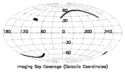
The EDR contains 462 square degrees of imaging data in five bands, and 54,008 spectra in that same area. The data were acquired in three regions: along the celestial equator in the Southern Galactic sky; along the celestial equator in the Northern Galactic sky; and in a region overlapping the SIRTF First Look Survey.
Table summarizes the imaging data included in the EDR. The ``run number'' is a designation we use for one continuous scan of the SDSS imaging camera on the sky, and a ``stripe'' is the great circle covered by a run, 2.5° wide. We cover each ``stripe'' in two ``strips'', separated in the north/south direction so that the interleaved scans of the six columns of the imaging camera completely cover the ``stripe.'' We define the great circles for the imaging survey in section 3.2.2. The location of each run and the effective area covered are indicated in the table. Runs 94/125 and 752/756 are long stripes on the equator, in the Southern and Northern Galactic caps, respectively, while runs 1336/1339 and 1356/1359 are shorter scans, off the equator, designed to overlap with the SIRTF First Look Survey. The sky coverage of the resulting imaging and spectroscopic data are illustrated in Figures 2.1 and 2.1.
|
|
|
|
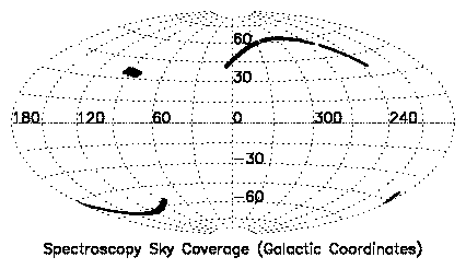
Table summarizes the spectroscopic data. As discussed in section 4.8, we select objects detected in the imaging data for spectroscopic observations. The nominal exposure time for each plate is 45 minutes, which typically yields a signal-to-noise ratio of 4.5 per pixel for objects with a g* magnitude of 20.2. The measured signal-to-noise ratio at g* = 20.2 for each plate is included in Table . For completeness, we list several plates which were designed but not unobserved; they have no entry in the (S/N)2 column.
The overall quality of the EDR is summarized briefly in Table .
2.2 Data Products
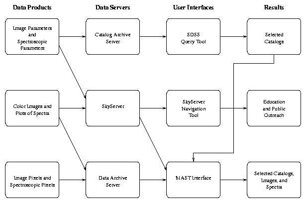
Figure summarizes the data products for imaging and spectroscopy, the three database servers we use to present these products to the astronomical community, and the user interfaces we have developed to help astronomers work with the data effectively. The data products described below are:
|
| Figure 3: Overview of data products and distribution for SDSS EDR. The left column contains all of the data products available. The second column contains the servers that hold data. Note that not all data products are contained in each of the servers. The third column contains the interfaces we provide to these servers. Choose which interface to use based on the results you wish to obtain, listed in the fourth column. |
- Image Parameters: the positions, fluxes, and shapes of all detected objects;
- Spectroscopic Parameters: the redshift, spectral classification, and detected lines of each spectrum;
- Color Images: JPEG images constructed from the g, r and i imaging data;
- Images: FITS image files of the corrected frames (§ 3.5) in five bands; a mask which records how each pixel was used in the imaging pipelines; 4×4 binned images of the corrected frames after detected objects have been removed; ``atlas'' images, which include all significant pixels around each detected object; and a GIF image of each spectrum, with features identified;
- Spectra: the flux- and wavelength-calibrated, sky-subtracted spectra, with error and mask arrays;
- Other Data Products: the number of objects loaded in the databases, summaries of observing conditions for imaging fields and for spectroscopic plates, and a variety of others.
2.2.1 Parameters, Classes, and Associations
We organize our measured parameters, for imaging and spectroscopic data, by grouping related parameters into classes. Table lists the classes. Tables , , , , , , , , and list the parameters in each class with a brief description.
In each table, we list the parameter name (in many cases, parameters have several synonyms, as listed), the datatype, a brief description, and, for Table , an indication of whether this is a tagged entry (a parameter for which searches are particularly fast; see § 2.4.1). For binary flags, the meaning of the bits are given explicitly. Parameters for which there exists a placeholder in the database, but are not yet calculated, are indicated as such with the phrase ``(placeholder)'' in the table.
Many quantities are defined for each band, and thus have five entries. In the Catalog Archive Server (§ 2.3.1) these are indexed with 0, 1, 2, 3, 4 inside of square brackets, [], for u,g,r,i,z, respectively. In the skyServer (§ 2.3.3) these are indexed with _u, _g, _r, _i, _z for the filters.
Some parameters are associations to objects in other classes. For example, an object in the class SpecObj (Table ) has a parameter plate, which is an object in the Plate class (Table ). This contains information common to the 640 spectra taken in one set of observations for the plate. The association is indicated in the table in the type column as OneAssoc(Plate). Other associations point to many (rather than one) objects. In SpecObj, for example, the parameter emissionredshift has the type ManyAssoc(EmissionRedshift). It points to a list of redshifts measured. The ``best'' value of the emission and absorption redshift is stored in z of SpecObj, but for complex spectra, you may access the full list of redshifts measured during processing.
2.2.2 Imaging Data Products
Image Parameters
The results of the imaging pipelines (described below in § 4.4) are summarized in Table , and the apertures used for radial profile measurements are in Table . For each object, we measure the position, several varieties of the flux, morphological parameters, and a provisional classification. We also include informational flags on each pixel in the images (Table ) and each object (Table ) and summary flags and statistics for each field (Table ). The choice of flags and which measure of flux and shape to use are dictated by the science goals of the SDSS. The catalog contains over 120 parameters and flags measured for 13,804,448 objects. 10,947,783 of these are unique, well-measured astrophysical objects.
The SDSS object catalogs are matched against the FIRST [Becker, White, & Helfand, 1995], ROSAT [Voges et al., 1999], and USNOA2.0 [Monet, 1998] databases; the resulting parameters are described in Table .
Images
Each corrected frame is a FITS image for one filter, 2048 columns × 1489 rows, with row number increasing in the scan direction. These are the imaging frames with flat field, bias, cosmic ray, and pixel defect corrections applied. A raw image contains 1361 rows, and a corrected frame has the first 128 rows of the following corrected frame appended to it. The pixels subtend 0.396˘˘ square on the sky.
Header information using the World Coordinate System (WCS) [Calabretta & Greisen, 2001] allows standard astronomical FITS tools to convert pixel position to (a,d) (§ 4.2.2).
Binned Images
Each file is a FITS image for one filter, 512 ×372 pixels, with WCS information. These are the corrected frames with detected objects removed and binned 4 ×4 pixels.
Mask Frame
Each file is a binary FITS table for one filter. Each row of the table describes a set of pixels in the corrected frame, using mask values described in Table .
Atlas Image
For each detected object, the atlas image comprises the pixels that were detected as part of the object in any filter. These are provided through a database, as either a JPEG color image, or as a FITS file for each selected filter.
Color Image
We combine the corrected frames from the g, r and i filters and produce a color image with the filters corresponding to blue, green, and red, respectively. The intensity mapping of each color is adjusted to enhance the appearance of these images. We use the same mapping for all of the color images.
2.2.3 Reading SDSS Binary Tables
Most of these files are simple FITS binary tables or images; The exceptions are Atlas Images (fpAtlas), Mask Frames (fpM), and PSF description files (fpField) files. We provide stand-alone code on our web site to enable you to interpret these files and read them into your own code.
2.2.4 Spectroscopic Data Products
Calibrated Spectra
These are the (l, flux) pairs that comprise the spectrum. The spectra are given in vacuum wavelengths in the heliocentric frame, with flux density given in units of 10-17 erg s-1 cm-2 Å-1. An estimated error is also output, as well as a mask associated with each pixel, as described in Table .
Spectroscopic Parameters
Catalogs produced by the spectroscopic pipelines (described below in § 4.10) are summarized in Tables and . For each spectrum, we measure the redshift using several techniques, locate and characterize lines, and assign an identification. The catalog contains 54,008 spectra, with 46 parameters measured for each spectrum, and 34 parameters measured for each emission line identified in each spectrum.
Images of the Spectra
For convenience, we also provide a plot of each spectrum. These are GIF images of the spectrum, with significant features, our classification, and measured redshift indicated.
2.2.5 Other data products
Table summarizes parameters that record the number of objects loaded in the database. Table summarizes data that describe the imaging data. A run, as already described, is all the data from a single contiguous scan of the imaging camera. These are combined into chunks, contiguous areas of the sky from which spectroscopic targets will be selected and spectroscopic tiling (the process by which targets are assigned to spectroscopic plates) will be done. A segment is a single piece of a run for a single camera column. The contiguous stream of data is divided into a series of fields (§ 3.5), whose detailed properties are also given in Table , including astrometric calibrations (§ 4.2), and details of the point-spread-function fitting (§ 4.3). Finally, the details for each spectroscopic plate are also given in Table .
Table lists constants we use to define the survey.
2.3 Database Servers
We have constructed three database servers to hold the imaging and spectroscopic data for the EDR, as shown in Figure . The Catalog Archive Server contains the measured parameters from all objects in the imaging survey and the spectroscopic survey. These are loaded in a database server we built using Objectivity, a commercial, object-oriented database server [Objectivity Inc., 2001]. The skyServer contains identical information, but it is loaded in a database server we built using a commercial, relational database server, SQLServer [Delaney, 2001]. The Data Archive Server contains the rest of the data products for the EDR, such as the corrected imaging frames, which are available for direct download, and the calibrated spectra, which are loaded in an Objectivity database.
2.3.1 Catalog Archive Server
The Catalog Archive Server is indexed to allow efficient queries on quantities commonly used in astronomical research (position, and magnitudes in our five filters). It also allows algebraic combinations of these quantities to be used in the queries. We have written a unique and powerful database server which allows users to make sophisticated queries efficiently. The general strategy of compiling a large astronomical database is described in Szalay et al. [2001], and our method of dividing the celestial sphere into a hierarchical triangular mesh, which enables efficient access based on position, is described in Kunszt et al. [2000]. The database server software is described in Thakar et al. [2000].
2.3.2 Data Archive Server
Given a set of object coordinates, either from the catalog archive server or some other source, the data archive server makes the detailed data (corrected frames, binned images, mask images, atlas images, color images, spectra, and spectral plots) available. It is not practical to access all of the imaging data in this way, but it does give convenient access to any selected field or spectrum contained in the EDR.
2.3.3 skyServer
The skyServer is a relational database server. Its language is not as rich as that provided by the catalog archive server, but it works well for many queries. This server was originally developed with outreach and education in mind, but it is also very useful for astronomical research.
2.4 User Interfaces
There are three separate user interfaces to the SDSS EDR, as shown in Figure .
We expect that typical users interested in extracting subsets of our imaging catalog based on position, flux, and colors, will find the MAST interface to the skyServer most useful. Sophisticated queries on flags and algebraic combinations of parameters are best done with the SDSS Query Tool (sdssQT). Users who wish to download atlas images, corrected frames, or spectra, should do so with the MAST interface to the data archive server.
2.4.1 SDSS Query Tool (sdssQT)
The sdssQT is a stand-alone application to manage and perform catalog archive server queries, and is available for download from our web sites, along with a detailed user's manual. The discussion that follows is a brief introduction to its use, to illustrate its capabilities. There are options to choose the output format (ASCII or binary), facilities to save queries, a simple text editor to create and modify queries, and communication with the Catalog Archive Server to follow the progress (and predict the time to completion) of active queries. An additional tool converts our binary output format to a FITS binary table.
The query language we developed is very similar to the Structured Query Language (SQL). The sdssQT includes several example queries, and the online user's guide provides additional explanations of the language and how to use it efficiently. The use of associations (§ 2.2.1) provides a powerful way to extract object data from many different classes simultaneously. Similarly, the inheritance properties of classes and their subclasses makes queries written for a given class run on all of its subclasses or sibling classes.
The grammar of this language is to select a set of parameters from a class that satisfy specified conditions. The SDSS Query Tool allows full access to all of the classes and parameters in the Catalog Archive Server. For example, the query:
SELECT ra,dec FROM SpecObj WHERE (z > 2)returns the parameters ra and dec (right ascension and declination) for all spectroscopic objects (i.e., from the class SpecObj) with redshift greater than 2.
One class must appear in the WHERE clause. One or more of the parameters from the classes may be listed in the SELECT clause and used in the WHERE clause, as long as they are included in the class mentioned in the FROM clause.
The PhotoObj class, containing the detected objects in the images, has the most entries, over 13 million. To facilitate selecting from these entries, we have designated a subset of the most commonly used parameters in the PhotoObj class to be part of a special class called Tag. The final column of Table indicates which parameters are in the Tag class. The database is structured in such a way that searches that select on these Tag parameters run significantly faster.
Additionally, many of the classes, like Tag, have numerous subclasses (Primary, Secondary, Galaxy, Star), described in the above mentioned tables. These subclasses all inherit the properties of the umbrella class. The same parameters are available in the subclasses as in the umbrella class, but they will be faster to query as each contains only a portion of the total objects. For example, users wanting data only on galaxies can execute queries on the Galaxy class; this avoids having to specify that objType=Galaxy if it were run on the entire Tag class, and will run faster as fewer objects are searched.
To access associated, or linked parameters, we use the ``.'' modifier. For example, spectroscopic objects from the SpecObj class all have a link back to the photometric object in the Tag class. This allows retrieval of parameters from both classes simultaneously. Use the syntax tag.r, for example, to obtain a spectroscopic target's r* magnitude. In Table , the parameter phototag has type OneAssoc(PhotoTag), so the query
SELECT ra,dec,phototag.r FROM SpecObjreturns the position and r* magnitude for all objects with spectra.
Some associations tie many objects in a class to one object of another class. For example, there can be many lines measured in one spectrum. The parameter measured in the SpecObj class has the type ManyAssoc(SpecLine). The following Association Query returns parameters for all of the lines of the selected spectrum:
SELECT name.name,wave,ew FROM
(SELECT measured FROM SpecObj WHERE
	plate.plateID == 384 && fiberID == 284)
The online user's guide to the SDSS Query tool contains a detailed description of the language, examples to help construct advanced queries, and details about macros to perform logical and arithmetic operations within queries.
2.4.2 MAST SDSS skyServer Interface
This provides a familiar interface to the object catalog, as it is based on the MAST interface6 which also serves catalogs from NASA missions and other surveys: GSC, DSS, and VLA-FIRST. This is the interface most will prefer for straight-forward queries based on (a,d). Objects that satisfy the query can be used one of several ways. The list may also be written to a comma-delimited text file, to be read by external programs, such as Microsoft Excel. The list may be written as a FITS binary table. Finally, the list may be browsed as an HTML table, where specific objects and data products (e.g. the corrected frame for the object, or the spectra for those objects with spectra) are then selected for use by the Data Archive Server.
2.4.3 MAST SDSS Data Archive Server Interface
The SDSS Image Products interface accepts a list of objects specified in one of the following formats: run/rerun/camcol/fieldID/objectID (see § 4.4.1), long object ID (from the skyServer or Catalog Archive Server), ra/dec, NED, or SIMBAD target names. Files generated by the sdssQT may be uploaded directly. All imaging products (atlas images, corrected frames, reconstructed frames, binned images, fields summaries, and mask files) are available. All of the files for a request are bundled together in a .tar, .tar.gz, or .zip file.
An object list from the MAST skyServer Interface can be sent to the data product interfaces via a ``shopping cart.'' To demonstrate this access, we begin in the MAST SDSS skyServer Interface. Select galaxies within 10 arcmin of (a,d)=(0,0) and 16 < r* < 17 by entering the coordinates in the RA,DEC boxes, 10.0 in the Radius(arcmin) box, highlighting GALAXY from the Object Type list, and by entering 16..17 in the Magnitude box for r. Three objects are returned. Choosing the ``Browse Results as HTML'' button brings up a list of these objects. Select the three objects by using the button in the Mark column, select Add marked records to shopping cart, and then select Retrieve data products for shopping cart. The data products may then be downloaded.
2.5 Access to Files
Data products are also available directly from the data archive server. Sophisticated users may want to download some of these files directly, but we consider these files to be intermediate data products, and focus our support and documentation efforts on the database servers and interfaces we described above. The data model, which describes the file naming conventions and FITS headers, is available on our web site.
2.5.1 Imaging Files
Image data are available from the main Data Archive Server page. Data for individual runs are in subdirectories specified by $run/$rerun, where valid $run/$rerun combinations for the EDR are 94/7,125/7, 752/8, 756/8, 1336/2, 1339/2, 1356/2, and 1359/3. Corrected frames are accessed under this root URL via
corr/$camCol/fpC-$run-$rerun-$filter$camCol-$field.fit.gz,where $camCol is the camera column (1 through 6), $run is the run number (6 digits with leading zeroes), $filter is the filter name (u, g, r, i, z), and $field is the field number (4 digits with leading zeroes). Binned images are accessed in a similar fashion, via
objcs/$camCol/fpBIN-$run-$filter$camCol-$field.fit.gz,as are the Mask images, via
objcs/$camCol/fpM-$run-$filter$camCol-$field.fit
The fpAtlas files in that same directory contain all of the atlas images for each field, but it is generally more convenient to access them with the Data Archive Server.
The catalogs of detected objects for each field are accessed via
objcs/$camCol/fpObjc-$run-$camCol-$field.fitbut these files do not yet include photometric or astrometric calibration.
Summary information for each field processed is accessed via
objcs/$camCol/fpFieldStat-$run-$camCol-$field.fitand results of the psp pipeline, which characterizes the point spread function for a field (§ 4.3), are accessed via
objcs/$camCol/fpField-$run-$camCol-$field.fit
2.5.2 Spectroscopy Files
Spectroscopy files are available from the main Data Archive Server page. Data for individual plates are in subdirectories specified by $plate/$mjd, where valid $plate/$mjd combinations are in Table .
Calibrated spectra which have been extracted from the spectroscopic frames with the spectro2d pipeline (§ 4.10.1) are available under the root URL via
2d_10/$plate/2dmerge/spMerge2d-$mjd-$plate-$fiber.fit,where $plate is the plate number (four digits, zero padded), $mjd is the date observations were completed (Table ), and $fiber is the fiber number (three digits, zero padded).
Calibrated spectra, with information from the spectro1d pipeline (§ 4.10.2), such as redshift and identification, are available under this root URL via
1d_10/$plate/1d/spSpec-$mjd-$plate-$fiber.fit.
2.6 User Support
We provide help for users at several levels. This paper is a general introduction to the data products. Our web sites have additional documentation. We maintain a set of frequently asked questions with answers to help people become more familiar with how to use the data set. There are also two mailing lists which we encourage users to join. The first is a SDSS Early Data Release Users' Group which we will use to communicate periodically with users. The second is the SDSS Early Data Release Users' Forum, where we encourage all users to post questions and suggestions. We will monitor this mailing list and post answers, or pointers to online documentation, as appropriate. We also support a help desk, which is accessible via email and telephone, as detailed on our web sites.
2.7 Acknowledging SDSS Data
Access to the SDSS EDR is open. These data may be used for any astronomical research. Data from the SDSS public archive may not be used for any commercial publication or other commercial purpose except with explicit approval by the Astrophysical Research Consortium.
Non-commercial and technical publications based on the SDSS EDR should contain the following acknowledgement:
``Funding for the creation and distribution of the SDSS Archive has been provided by the Alfred P. Sloan Foundation, the Participating Institutions, the National Aeronautics and Space Administration, the National Science Foundation, the U.S. Department of Energy, the Japanese Monbukagakusho, and the Max Planck Society. The SDSS Web site is http://www.sdss.org/.
The Participating Institutions are The University of Chicago, Fermilab, the Institute for Advanced Study, the Japan Participation Group, The Johns Hopkins University, the Max-Planck-Institute for Astronomy (MPIA), the Max-Planck-Institute for Astrophysics (MPA), New Mexico State University, Princeton University, the United States Naval Observatory, and the University of Washington.''
3 Hardware
3.1 2.5m Telescope and Instruments
The telescope and its somewhat unusual optical design [Waddell et al., 1998] are described in detail in York et al. [2000] and the SDSS Project Book, available on the web7. The camera and the pair of double spectrographs are discussed there as well; see also Gunn et al. [1998]. We review here only details which are of direct relevance to working with the data.
3.2 Imaging System
The parameters of direct relevance to the imaging system of the SDSS are presented in Table . Since York et al. [2000] was published, we have learned a great deal about our filter and detector system, and a preliminary discussion of these matters is given below, as are some details concerning the geometry of the great-circle Time Delay Integration (TDI, or Drift Scan) stripes which cover the survey area.
3.2.1 Filters
The situation with the SDSS response functions for the five filter passbands, and the resulting photometric system, is rather complex. There is a set of primary standard stars which have been measured at the U. S. Naval Observatory 40˘˘ telescope and with the SDSS Photometric Telescope (§ 3.4) which together define a photometric system which we believe to be self-consistent to approximately 1%; this system is roughly as described in Fukugita et al. [1996]. These primary standards are described further in § 4.5 below. Unfortunately, the filters used on the USNO and PT telescopes differ systematically from those on the 2.5m camera, and we still do not have a complete understanding of the transformations between these two systems8. Thus the photometric system defined by the USNO and PT telescopes is not directly applicable to the 2.5m data, as described in detail in § 4.5. Figure 3.2.1 gives the average measured quantum efficiencies of the 2.5m camera detectors multiplied by the reflectivity of the primary and secondary (the two transmissive surfaces have negligible effect on the throughput); curves are given both assuming no atmosphere, and including the transmission of the atmosphere above Apache Point on a night of average humidity at airmass 1.3. Tables containing the system response in each filter are available on our web sites. The thinned CCDs also suffer from internal scattering that scatters light longward of roughly 6000Å into an extended halo around an object; this decreases the effective quantum efficiency for a point source. For extended sources (size > 30˘˘), this effect is negligible, and the dashed curves indicate the quantum efficiency in this case in the r and i filters. The z chip is thick, and does not suffer from this problem.
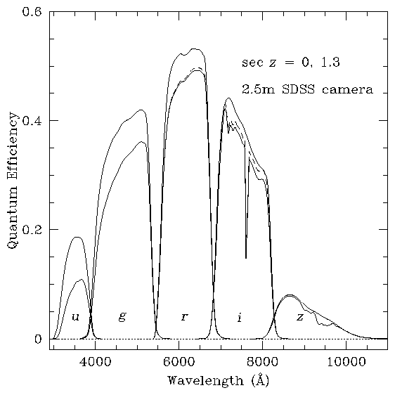
The camera responses were measured by an instrument with a roughly triangular wavelength response with FWHM about 100Å; this resolution has not been corrected for in these data but does not appreciably alter the shapes. Better and more detailed response data will be obtained and published later, but the results here are adequate for most purposes.
Table gives corresponding properties of
the filters, updating those tabulated in Fukugita et al. [1996] and
Fan et al. [2001a]: the effective wavelength of each filter leff, the
photon-weighted mean of the quantity ln2(l/leff)
(a measure of the effective width of the filter),
the Full Width at Half Maximum of the filter, and Q, the integral of the
system efficiency over d(lnl), effective quantum
efficiency (all assuming 1.3 airmass, and observing a point source). This
last quantity relates the measured apparent magnitude (on an AB
system) to the number of detected electrons:
| (1) |
As pointed out in § 1, we refer to data on the standards system with the magnitude labels (u˘g˘r˘i˘z˘) and the provisional 2.5-meter magnitudes with the labels (u* g* r* i* z*). The SDSS photometry itself is presented in the provisional 2.5-meter system. Finally, the 2.5-meter filters themselves are referred to in this paper simply as u, g, r,i, and z, a change from some of our earlier papers.
3.2.2 Great Circle Drift Scanning
The survey coordinate system (l,h) is a spherical coordinate system with poles at a2000 = 95\arcdeg, d2000 = 0\arcdeg and a2000 = 275\arcdeg, d2000 = 0\arcdeg. The survey equator is thus a great circle perpendicular to the J2000 celestial equator, intersecting it at a2000 = 185\arcdeg and a2000 = 5\arcdeg. Lines of constant h are great circles perpendicular to the survey equator and lines of constant l are small circles parallel to the survey equator. l = 0\arcdeg, h = 0\arcdeg is located at a2000 = 185\arcdeg, d2000 = 32.5\arcdeg, with h increasing northward.
The survey area is divided into stripes, where each stripe is centered
along a line of constant h, separated from the adjoining
stripe(s) by 2.5 \arcdeg. Each drift scan tracks a survey stripe,
offset by ±386 arcsec perpendicular to the stripe. Two scans (or
``strips''), one offset to the north and one to the south, are
required to fill a stripe.
The survey latitude tracked by stripe
n is given by
| (2) |
| (3) |
The natural coordinate system to use for processing a given drift scan is the great circle coordinate system for that stripe, (m,n), in which the equator of the coordinate system is the great circle tracked by the scan. This great circle is inclined by i = h+ 32.5 \arcdeg to the J2000 celestial equator, with an ascending node of 95 \arcdeg. m = a at the ascending node. m increases in the scan direction (east) and n increases to the north. Each stripe has its own great circle coordinate system.
For reference, the equations to transform among the different coordinate systems are:
|
3.3 Spectroscopic System
We produce 640 individual spectra in a three degree diameter field at a resolution R ş l/Dl of about 1800 in the wavelength range of 3800 to 9200 Å. This wavelength range is divided between two cameras by a dichroic at about 6150 Å, and there are two spectrographs, each producing 320 spectra. There are thus 4 CCD detectors, each of the same kind as are present in the g, r, and i bands in the camera, 2048 pixels square with 24 micron pixels. The spectroscopic system is discussed in York et al. [2000]. Results from commissioning the system are discussed in Castander et al. [2001].
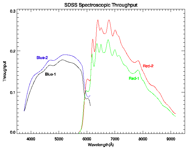
The fibers carrying the light from the drilled plug-plates to the spectrographs subtend about 3 arcseconds in the focal plane, and are imaged in turn in the spectrograph cameras with a footprint of about 3 pixels. The straight-through transmissive immersion grisms produce a dispersion which is roughly linear in log wavelength. The spectrographs are very efficient; quantum efficiencies on the sky as measured from standard stars as a function of wavelength for each of the four spectrographic CCDs are presented in Figure 3.3. They peak at over 25% in the red, and just under 20% in the blue.
The nominal exposure time for each plate is 45 minutes, split into at least three parts for cosmic ray rejection, with the exact number determined by observing conditions. This set of science exposures is preceded and followed by a series of shorter exposures for calibration: arcs, flat-fields, and a 4-minute smear exposure on the sky for spectrophotometric calibration, in which the telescope is moved so that the 3 arcsec fiber on each object effectively covers a 5˘˘×8˘˘ aperture, aligned with the parallactic angle. The smear exposures allow us to account for object light excluded from the 3 arcsec fibers due to seeing and atmospheric refraction; they provide an accurate (albeit low signal-to-noise ratio; S/N) measure of the true spectral shape of the objects and are used for spectrophotometric calibration9. The calibration and science exposures are immediately processed through a streamlined version of the 2d spectroscopic pipeline (§ 4.10) to inform the observers whether the calibrations were successful and to provide S/N diagnostics on the science exposures.
For each science exposure, the (S/N)2 per pixel through the SDSS imaging passbands is measured and evaluated as a function of fiber magnitude for each spectrograph camera. We take repeated 15-minute exposures until the cumulative median (S/N)2 > 15 at g*=20.2 and i*=19.9 in all 4 cameras. In clear, non-moony conditions, the (S/N)2 threshold is easily reached in 3 exposures, and we never take fewer than three exposures; in (partially) cloudy or moony conditions, more exposures may be required.
3.4 Photometric Telescope
We use a 20-inch Photometric Telescope, located next to the 2.5-meter telescope's enclosure, to measure nightly extinctions and to observe transfer fields (secondary patches) that in turn are used to calibrate the 2.5-meter imaging data. Details of the full photometric calibration process can be found in § 4.5. This telescope is a commercial reflector built by DFM Engineering (Longmont, Colorado), modified to incorporate improved baffling and a coma corrector to increase its field of view. It is equipped with a thinned SITe 2048×2048 chip with 24 micron square pixels like the u chips in the 2.5m camera, and a set of filters nominally the same as those in the camera. Please refer to § 3.2.1.
The telescope operates automatically, observing primary standard stars and secondary patch transfer fields selected from an on-line database. Observing staff can monitor progress with real-time tools that display cloud cover, extinction coefficients, and observing progress [Hogg et al., 2001].
3.5 Data Acquisition
The data acquisition system [Petravick et al., 1994] records information from the imaging camera, spectrographs, and photometric telescope. Data are transferred via magnetic tape, with critical, low-volume samples sent over the internet. Each system uses report files to track the observations.
Data from the imaging camera are collected in the Time Delay Integration (TDI, or Drift Scan) mode. We treat the data from each imaging camera column of 5 photometric and 2 astrometric CCDs as a scan line. For convenience, data from each CCD are broken into frames containing 1361 lines. Before processing, the 128 rows from the next frame are added to the top of each frame, so that the pipelines work on 2048×1489 images. The resulting overlap between reduced frames (128 rows) is roughly the same as the number of columns that overlap with the other strip of a stripe. Some objects are detected in more than one frame, but when loading the databases we mark one of these detections as the ``primary'' detection (see the discussion in § 4.7 below). The frames which correspond to the same sky location in each of the five filters are grouped together for processing as a field. Frames from the astrometric CCDs are not saved, but rather stars from them are detected and measured in real time to provide feedback on telescope tracking and focus. These measurements are also written to magnetic tape. This same analysis is done for the photometric CCDs, and we save these results along with the actual frames. Each night, a special bias run is taken to monitor the bias levels on CCD amplifiers.
Data from the spectrographs are read from the four CCDs (one red channel and one blue channel in each of the two spectrographs) after each exposure. A complete set of exposures includes bias, flat, arc, smear, and science exposures taken through the fibers, as well as a uniformly illuminated flat to take out pixel-to-pixel variations.
Data from the photometric telescope include bias frames, dome and twilight flats for each filter, measurements of primary standards in each filter, and measurements of our secondary calibration patches in each filter.
All of these systems are supported by a common set of observers programs, with observer interfaces customized for each system to optimize our observing efficiency.
4 Software
4.1 Data Processing Factory
Data from APO are transferred to Fermilab for processing and calibration. Three flavors of data are produced at APO: data from the imaging camera, data from the Photometric Telescope, and spectra from the spectrographs. Imaging data are processed with the imaging pipelines: the astrometric pipeline (astrom; § 4.2) performs the astrometric calibration; the postage stamp pipeline (psp; § 4.3) characterizes the behavior of the point spread function as a function of time and location in the focal plane; the frames pipeline (frames; § 4.4) finds, deblends, and measures the properties of objects; and the final calibration pipeline (nfcalib; § 4.5.3) applies the photometric calibration to the objects. This calibration uses the results of the photometric telescope data processed with the monitor telescope pipeline (mtpipe; § 4.5.2). The combination of the psp and frames pipelines is sometimes referred to as photo.
Individual imaging runs which interleave are prepared for spectroscopy with the following steps: resolve (§ 4.7) selects a primary detection for objects which fall in an overlap area; the target selection pipeline (target; § 4.8) selects objects for spectroscopic observation; and the plate pipeline (plate; § 4.9) specifies the locations of the plates on the sky, and the location of holes to be drilled in each plate.
Spectroscopic data are first extracted and calibrated with the 2d pipeline (spectro2d; § 4.10.1), and then classified and measured with the 1d pipeline (spectro1d; § 4.10.2).
The EDR was prepared using the versions of pipelines indicated in Table . The data for the EDR were reduced with a consistent set of pipeline versions, with only minor version changes to address operational issues.
We continue to develop these pipelines, and in what follows, we describe known problems and future developments where relevant. We also continue to improve photometric calibration techniques (§ 4.5).
4.2 Astrometric Pipeline
A separate great circle coordinate system is defined for each stripe (§ 3.2.2). In these systems, the stripe center is the equivalent of the equator in the equatorial (a,d) system. Pixel coordinates are corrected for empirically derived optical distortion terms, and the resulting mapping from corrected CCD row and column pixel positions to great circle longitude and latitude is linear to very good approximation. Astrometric solutions are carried out in this coordinate system. One of two reduction strategies is employed depending upon the coverage of astrometric catalogs:
- Whenever possible, stars detected on the r photometric CCDs are matched directly with stars in the USNO CCD Astrograph Catalog (UCAC) [Zacharias et al., 2000]. UCAC extends down to R = 16, giving approximately 2 magnitudes of overlap with unsaturated stars on the photometric r CCDs. For the EDR, this technique was used for the south equatorial stripe (runs 94 and 125) and for the north equatorial stripe (runs 752 and 756).
- If UCAC coverage is not available to reduce an imaging run, bright stars detected with the astrometric CCDs are matched with the Tycho-2 catalog [Høg et al., 2000]. The fainter stars on the astrometric CCDs are then matched with the brighter detections on the r CCDs, enabling us to transfer the pixel coordinates of the catalog stars onto the r CCD coordinate system. In the EDR, this technique was used for the SIRTF area, runs 1336, 1339, 1356, and 1359.
For each r frame, these mappings result in an affine transformation relating corrected pixel positions to celestial coordinates. A secondary catalog is produced from the detections on the r CCDs. This secondary catalog is then matched to centroid positions on the i, u, z, and g CCDs to derive affine transformations in those filters. The transformation also includes terms to correct for differential chromatic refraction and those terms are applied when the colors of objects are known (Table ). Positions of detected objects given in this EDR have had this correction applied.
4.2.1 Astrometric Quality
The relative astrometry between the r and the i, u, z, and g CCDs is independent of the astrometric catalog used, and typically has rms errors of 20 to 30 mas per coordinate, and systematic errors of order 20 mas. The quality of the absolute astrometry (based on the r astrometric solutions and centroids) is dependent on the astrometric catalog used, and is dominated by systematic errors which vary on timescales of minutes. Within a given run, the distribution of systematic errors is well characterized by a Gaussian. Reductions against UCAC have rms systematic errors of order 50 mas per coordinate. Reductions against Tycho-2 have rms systematic errors of order 100 mas, and show additional systematic errors constant over entire scans of up to 50 mas. Centroiding errors contribute an additional random source of error, of order 20 mas, for objects brighter than r* = 20. Comparison with the astrometry of the Two-Micron All Sky Survey for stars in common shows systematic offsets under 50 mas, well within our quoted errors and the expected systematic astrometric calibration effects quoted by the 2MASS team.
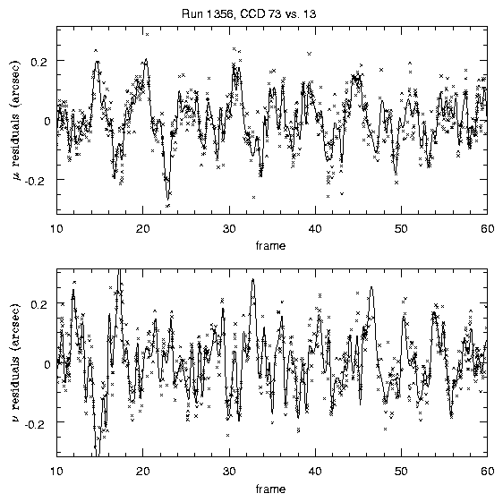
Atmospheric conditions contribute significantly to image wander. These affect the Tycho-2 reductions more than the UCAC reductions due to the shorter integration times on the astrometric CCDs. We attempt to follow this wander by fitting the residuals with cubic splines. Figure 4.2.1 shows the astrometric residuals as a function of frame number for a typical run. The spline-fitted solution is superposed on the points showing the residuals. The top plot shows m residuals (along the direction of the scan), and the bottom plot shows n residuals (the cross-scan direction). Approximately 100 frames per hour are obtained, so the figure shows roughly half an hour of scanning. Note that the residuals wander several tenths of an arcsecond over time scales of minutes. The frequency and amplitude of these wanderings vary from night to night (and, occasionally, hour to hour).
4.2.2 WCS
The bias-subtracted, flatfielded data frames in the EDR include World Coordinate System (WCS) information in the FITS file headers. This information enables some display and analysis software to provide RA and DEC information on a pixel by pixel basis and also to overlay an equatorial coordinate grid over the image.Present WCS proposed standards [Calabretta & Greisen, 2001] do not fully support a rigorous transformation from great circle to equatorial coordinates. As a result, the WCS representation does not reflect the full accuracy of the astrometric solution, but the accuracy is better than one pixel (about 0.4˘˘) within a frame.
The conversion from (row,col) measured in a field to (a,d)(J2000
degrees) is
|
4.3 The Postage Stamp Pipeline
As mentioned above, the data stream from each CCD is divided into an overlapping series of 10˘×13.5˘ frames, for ease of processing; the frames pipeline (§ 4.4) will process these separately. However, in order to ensure continuity along the data stream, certain quantities need to be determined on timescales up to the length of the imaging run. The astrometric and photometric calibrations certainly fall into that category; in addition, the Postage Stamp Pipeline (psp) calculates a global sky for a field, flatfield vector, bias level, and the point-spread function (PSF).
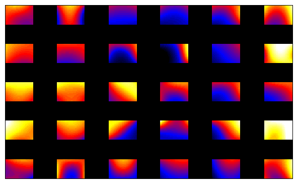
Even in the absence of atmospheric inhomogeneities, the SDSS telescope delivers images whose FWHMs vary by up to 15% from one side of a CCD to the other; the worst effects are seen in the chips furthest from the optical axis. Moreover, since the atmospheric seeing varies with time, the delivered image quality is a complex two-dimensional function even on the scale of a single frame. An example of the instantaneous image quality across the imaging camera is shown in Figure 4.3, where each rectangle represents one chip10.
The description of the point spread function (PSF) is critical for accurate PSF photometry, for star/galaxy separation, and for unbiased measures of the shapes of non-stellar objects; we need to map the full variation of the PSF even on scales of a single frame. The SDSS imaging PSF is modeled heuristically in each band using a Karhunen-Loève (KL) transform [Lupton et al., 2001c]. In particular, using stars brighter than roughly 20th magnitude, we expand the PSF from a series of five frames into eigen-images, and keep the first three terms. We fit the variation of the coefficients multiplying these terms to second order in position across the chip, using data from the frame in question, plus the immediately preceding and following half-frames.
The success of this KL expansion is gauged by comparing PSF photometry based on the modeled KL PSFs to large aperture photometry for the same (bright) stars. The width of the distribution of these differences is typically 1% or less, which is thus an upper limit on the accuracy of the PSF photometry (not including calibration problems; see § 4.5). Without accounting for the spatial variation of the PSF across the image, the photometric errors would be as high as 15%. We have recently found a subtle dependence of the PSF width on stellar color in the g band; this affects PSF photometry at the < 2% level, and will be addressed in future data releases.
Parameters that characterize one frame of imaging data are stored in the class Field (Table ). The status parameter flag for each frame indicates the success of the KL decomposition; its possible values are given in Table . In particular, if the data do not support the fitting of a second-order term to the variation of the coefficients with position, a linear fit is carried out, and status is set to 1. If even this is not warranted by the data, the coefficients are set to be constants, and the status flag is set to 2. Finally, if no PSF stars are available at all, the PSF model is set to that of the previous frame, and status = 3. A more quantitative measure of the accuracy of the PSF fit on a given frame is given by the scatter in the difference between PSF magnitudes and aperture magnitudes, as reported in psfApCorrectionErr. Note that the actual KL values and the eigenshapes are not reported in the tables, so the shape of the PSF as a function of position within a CCD cannot be reconstructed based on the parameters included in this EDR.
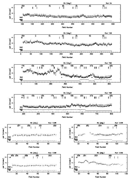
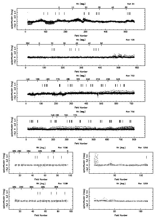
The psp returns various measures of the PSF shape in addition to the KL decomposition, including parameters of the best-fit double-Gaussian, evaluated at the center of each frame. These are the psf2GSigma parameters in the Field class. The psfWidth is is the effective width also determined at the center of each frame. It is a good generic number to quote for the seeing on each frame. Figure 4.3 shows the psfWidth in r for each CCD column in each run of the EDR imaging data. Improvements in telescope collimation and thermal environment since these data were taken have given rise to substantially better seeing.
The psp calculates a PSF aperture correction for each field. We did not fully test this correction and did not properly apply it to the EDR. The quantity apCorrRunErr is the median value of the difference between psfMag and the aperture magnitude measured with a 7.43\arcsec radius aperture over the bright stars in the frame, and is a measure of the limitations of our KL decomposition of the PSF. This quantity is Gaussian-distributed with sapprox. 0.03 mag, but apCorrRunErr can be as large as 0.1 mag in regions that the PSF is changing rapidly (FWHM changing by > 10% on a single frame); adding it directly to the psfMag in the EDR improves the overall PSF photometry accordingly. This correction will be applied to the data correctly in future data releases of the SDSS data. apCorrRunErr is shown for each run in Figure 4.3, and we provide a table of these corrections on our web site.
4.4 The Frames Pipeline
The frames pipeline (frames) detects, deblends, and measures objects, carrying out this processing on a field-by-field basis. This section describes what one needs to know to interpret the quantities we calculate in frames, rather than the technical details, which will be covered in Lupton et al. [2001b]. These quantities are stored in the PhotoObj and Profile classes (Table ). Mask bits set in objFlags of PhotoObj are for the object detections for all bands combined. Mask bits set in flags of PhotoObj are for the detection in each band. The mask bit values are given in Table . We refer to these classes and masks throughout this section. Further products of the imaging pipelines are given in § 2.2.
4.4.1 How frames Designates Objects
Each object detected during the frames analysis of a particular set of data is given a unique identifier which consists of five integers:
- run of class Segment (Table ): A run number refers to a given uninterrupted drift-scan.
- rerun of class Segment (Table ): Each time we analyze a run with a different set of pipeline version or calibrations we assign it a new rerun number. The same rerun number in different runs does not necessarily refer to the same version of the pipelines.
- camCol of class Segment (Table ): This number, from 1 to 6, refers to the dewar, or column of photometric CCDs in the imaging camera, by which this object was imaged.
- fieldID of class Field (Table ): Refers to which field (§ 3.5) the object is in.
- objID of class PhotoObj (Table ): This is an identification number for the object that is unique within each field.
Several different versions of the pipelines were run on the imaging data for the EDR (Table ). The rerun number for each run distinguishes a set of pipeline versions. Two rerun numbers are important for the EDR. The first rerun was used to select targets for spectroscopic observation. The second rerun used the most recent versions of the pipelines, and the results of this processing are distributed. Between reruns of frames, the run, camCol and fieldID of detected objects do not change, because frames acts on individual frames. However, the objID does change. Future data releases will most likely be made with yet another rerun which uses the most current version of our pipelines and calibrations.
In addition, data quality flags are set for each field, after we evaluate the processing from an entire run. These are discussed below in section 4.6.
4.4.2 Outline of frames
The pipeline analyzes the data one field (§ 3.5) at a time. Because information about each object is contained in five separate frames, one for each filter, the five frames for each field are processed together.
Each frame has instrumental signatures (flat field, bias, cosmic rays, and bad columns) removed, and the global sky value from the psp subtracted. The CCDs are known to be non-linear by of order 2% near saturation; this is not corrected for in the current version of the pipeline. Cosmic rays are found as objects with gradients between adjacent pixels substantially steeper than allowed by the PSF and are interpolated over. Note that our images are marginally well-sampled in 1˘˘ seeing. Previously recognized bad columns are interpolated over using linear prediction (e.g., Rybicki & Press 1992), as are bleed trails from saturated stars.
Objects containing a (found and interpolated-over) cosmic ray are flagged by having the mask bit CR set in flags for that band; objects with any interpolated pixels in them at all (due to bad columns or bleed trails) are flagged by having INTERP set. INTERP_CENTER indicates that a pixel was interpolated over within 3 pixels of the center of the object, and PSF_FLUX_INTERP indicates that at least 20% of the PSF flux is interpolated; in rare cases, photometry of objects with these latter two flags set might be suspect.
Next, objects in the frame are detected and their properties measured in a four step process in each band. First, an object finder is run to detect bright objects. In each band, the object-finder detects pixels which are more than 200s (corresponding roughly to r* = 17.5) above the sky noise; only a single pixel need be over this threshold for an object to be detected at this stage. These objects are flagged as BRIGHT. The extended power-law wings of BRIGHT objects which are saturated are subtracted from the frame. Such stars are marked SUBTRACTED. Then, the sky level is estimated by median-smoothing the frame image on a scale of approximately 100 arcsec; the resulting ``local'' sky image is subtracted from the frame (remember that a global sky determined on an entire frame has already been subtracted). This sky level is stored for each object for each band in the parameter sky (and an associated uncertainty skyErr), in units of asinh magnitudes (§ 4.4.5) per square arcsec. For children of blends (§ 4.4.3), the sky parameter includes the contribution of its siblings.
Third, we find objects by smoothing the image with a Gaussian fit to the PSF, and look for 5s peaks over the (smoothed) sky in each band. After objects are detected, they are ``grown'' more-or-less isotropically by an amount approximately equal to the radius of the seeing disk. We then define an object to be a connected set of pixels which are detected in at least one band. Note that all pixels in the object are subsequently used in the analysis in every band, whether or not they were originally detected in that band. The photometric pipeline never reports an upper limit for the detection of an object, but rather carries out a proper measurement, with its error, for each of the varieties of fluxes listed in § 4.4.5.
Objects detected in a given band at this stage are flagged by setting the mask bit BINNED1 (Table ) in flags of the PhotoObj class in that band. All pixel values in these BINNED1 objects are then replaced by the background level (with sky noise added in), the frame is rebinned into a 2×2 image, and the object-finder is run again. The resulting sample is flagged in a similar way with the BINNED2 mask, and pixel values in these objects are replaced with the background level. Finally, we rebin the original pixel data at 4×4, and objects found at this stage are flagged BINNED4. The set of detected objects then consists of all objects with pixels flagged BINNED1, BINNED2, or BINNED4.
Fourth, the pipeline measures the properties of each object, including the position, as well as several measures of flux and shape, described more fully below. It attempts to determine whether each object actually consists of more than one object projected on the sky, and if so, to deblend such a ``parent'' object into its constituent ``children'', self-consistently across the bands (thus all children have measurements in all bands). Then it again measures the properties of these individual children. Bright objects are measured twice: once with a global sky, and no deblending run; this detection is flagged BRIGHT, and a second time with a local sky. For most purposes, only the latter is useful, and thus one should reject all objects flagged BRIGHT in compiling a sample of objects for study.
Other flag bits listed in Table that are useful at this stage are:
- SATUR, indicating that at least one pixel in the object is flagged as saturated (the corresponding SATUR_CENTER indicates that the saturated pixel(s) are close to the center, to distinguish extended objects blended with saturated stars on their outskirts; unfortunately, this distinction is not as clean as we would like, due to improper handling of diffraction spikes).
- EDGE, indicating that the object overlaps the edge of the frame, which may affect the photometry of the object.
Finally, the pipeline outputs the measured quantities for each object, including all of the BRIGHT objects, all the parents, and all the children. In the following sections, we discuss how to interpret these outputs.
A typical frame at high Galactic latitudes contains of order 1000 objects, including of order 5 objects chosen deliberately in regions where no objects are detected; these are used to place sky fibers for spectroscopy, and are classified as Sky. Repeat observations of a given area of sky in roughly 1.5˘˘ seeing shows that our 95% completeness limit for stars is u*=22.0, g*=22.2, r*=22.2, i* = 21.3, and z* = 20.5; the completeness drops to zero over roughly half a magnitude. These numbers are somewhat worse than quoted in the SDSS Project Book [York et al., 2000], as that calculation assumed 1˘˘ seeing and slightly broader filters.
4.4.3 Deblending of Objects
Once objects are detected, they are deblended by identifying individual peaks within each object, merging the list of peaks across bands, and adaptively determining the profile of images associated with each peak, which sum to form the original image in each band. The originally detected object is referred to as the ``parent'' object and has the flag BLENDED set if multiple peaks are detected; the final set of sub-images of which the parent consists are referred to as the ``children'' and have the flag CHILD set. Note that all quantities in class PhotoObj (Table ) are measured for both parent and child. For each child, parent gives the id of the parent (for parents themselves or isolated objects, this is set to the id of the BRIGHT counterpart if that exists; otherwise it is set to -1); for each parent, nchild gives the number of children an object has. Children are assigned the id numbers immediately after the id number of the parent. Thus, if object with id 23 is set as BLENDED and has nchild equal to 2, objects 24 and 25 will be set as CHILD and have parent equal to 23.
The list of peaks in the parent is trimmed to combine peaks (from different bands) that are too close to each other (if this happens, the flag PEAKS_TOO_CLOSE is set in the parent). If there are more than 25 peaks, only the most significant are kept, and the flag DEBLEND_TOO_MANY_PEAKS is set in the parent.
In a number of situations, the deblender decides not to process a BLENDED object; in this case the object is flagged as NODEBLEND. Most objects with EDGE set are not deblended. The exceptions are when the object is big enough (larger than roughly an arcminute) that it will most likely not be completely included in the adjacent scanline either; in this case, DEBLENDED_AT_EDGE is set, and the deblender gives it its best shot. When an object is larger than half a frame, the deblender also gives up, and the object is flagged as TOO_LARGE. Other intricacies of the deblending results are recorded in flags listed in Table ; see Lupton et al. [2001b] for a complete description.
On average, about 15-20% of all detected objects are blended, and many of these are superpositions of galaxies which the deblender successfully treats by separating the images of the nearby objects. Thus, usually it is the childless (not BLENDED) objects which are of most interest for science applications. However, the versions of the pipelines used for the EDR occasionally deblends complex galaxies with large angular size, such as nearby face-on spiral galaxies, in a way which the human eye would tend not to. Thus, some care is required in the analysis of samples of bright and/or large objects in the survey. Later versions of the deblender handle these cases much more gracefully, and future data releases will incorporate these improvements.
4.4.4 Moving Objects
Main-belt asteroids have a proper motion of several arcsec in the roughly 5 minutes it takes for an object to cross the imaging camera. This means that they will have a different centroid in the different photometric bands. If not taken into account, this could mean that they would be deblended into separate objects of unusual color, playing havoc with the target selection algorithms (§ 4.8). Thus the deblender checks every object for consistency with uniform proper motion between the filters. In the PhotoObj class (Table ) the quantities colv and rowv (and their associated errors), give the resulting proper motion (along the columns and rows of the CCDs respectively) in units of degrees per day. The PSF photometry in each band is done on the object center, taking the motion into account, and therefore is properly measured [Ivezi\'c et al., 2001].
Flag bit values listed in Table describe this processing. The MOVED flag indicates that the deblender considered whether to deblend the object as moving; it is not very useful. If the deblender actually deblended the object as moving, the flag DEBLENDED_AS_MOVING is set; otherwise the flag NODEBLEND_MOVING is set. Note that an object can have a statistically significant motion without being deblended as such if the motion is small enough that the photometry would be fine without taking it into account. An object whose motion is not statistically significant is flagged STATIONARY, while an object whose motion is inconsistent with a straight line is flagged BAD_MOVING_FIT.
4.4.5 Measurements of Flux
We have discussed how frames detects, deblends, and designates objects. This section and the next discuss the measurements applied to each resulting object. Each of the quantities described here has an associated estimated error measured as well, unless otherwise mentioned. In this subsection, we discuss the various measurements made of the flux in each object.
We begin by describing the magnitude scale which the SDSS uses. Unless otherwise specified (the most important exceptions being petroMag and modelMag, to get self-consistent colors), the measures discussed here are applied independently in each band pass. Magnitudes within the SDSS are expressed as inverse hyperbolic sine (or ``asinh'') magnitudes, described in detail by Lupton, Gunn, & Szalay (1999). The transformation from linear flux measurements to asinh magnitudes is designed to be virtually identical to the standard astronomical magnitude [Pogson, 1856] at high signal-to-noise ratio, but to behave reasonably at low signal-to-noise ratio and even at negative values of flux, where the logarithm in the Pogson magnitude fails. This allows us to measure a flux even in the absence of a formal detection; we quote no upper limits in our photometry.
The asinh magnitudes are characterized by a softening parameter b,
the typical 1 s noise of the sky in a PSF aperture in 1'' seeing. The relation
between detected flux f and asinh magnitude m is (see equation (3) of ):
| (7) |
For isolated stars, which are well-described by the PSF, the optimal measure of the total flux is determined by fitting a PSF model to the object. In practice, we do this by sinc-shifting the image of a star so that it is exactly centered on a pixel, and then fitting a Gaussian model of the PSF to it. This fit is carried out on the local PSF KL model (§ 4.3) at each position as well; the difference between the two is then a local aperture correction, which gives a corrected PSF magnitude. Finally, we use bright stars to determine a further aperture correction to a radius of 7.4˘˘ as a function of seeing, and apply this to each frame for its seeing. This involved procedure is necessary to take into account the full variation of the PSF (measured in the psp described above) across the field, including the low signal-to-noise ratio wings. Empirically, this reduces the seeing-dependence of the photometry to below 0.02 mag for seeing as poor as 2˘˘. The resulting magnitude is stored in the quantity psfMag. As mentioned above, the flag PSF_FLUX_INTERP warns that the PSF photometry might be suspect. The flag BAD_COUNTS_ERROR warns that because of interpolated pixels, the error may be under-estimated.
The PSF errors include contributions from photon statistics and uncertainties in the PSF model and aperture correction, although they do not include uncertainties in photometric calibration (§ 4.5). Repeat observations show that these errors are probably underestimated by 10-20%.
The flux contained within the aperture of a spectroscopic fiber (3 arcsec in diameter) is calculated in each band and stored in fiberMag. Note that no correction for seeing is applied to this measure of the magnitude. For children of deblended galaxies, some of the pixels within a 1.5 arcsec radius may belong to other children. In this case, the fiber magnitudes can be rather misleading, as they will not reflect the amount of light which the spectrograph will see. For future data releases, we will calculate the true flux within a fiber diameter, including all light from the parent that falls in the aperture centered at the location of the child. We will also correct the detected flux to a fiducial value of the seeing.
For galaxy photometry, measuring flux is more difficult than for stars, because galaxies do not all have the same radial surface brightness profile, and have no sharp edges. In order to avoid biases, we wish to measure a constant fraction of the total light, independent of the position and distance of the object. Please refer to the discussion in Strauss et al. [2001]. To satisfy these requirements, the SDSS has adopted a modified form of the Petrosian [1976] system, measuring galaxy fluxes within a circular aperture whose radius is defined by the shape of the azimuthally averaged light profile.
We define the ``Petrosian ratio'' RP at a radius r from
the center of an object to be the ratio of the local surface
brightness in an annulus at r to the mean surface brightness within
r, as described by Blanton et al. [2001a],Yasuda et al. [2001],Strauss et al. [2001]:
| (8) |
The Petrosian radius rP is defined as the radius at which
RP(rP) equals some specified value RP,lim, set
to 0.2 in our case. The
Petrosian flux in any band is then defined as the flux within a
certain number NP (equal to 2.0 in our case) of r Petrosian radii:
| (9) |
The aperture 2 rP is large enough to contain nearly all of the flux for typical galaxy profiles, but small enough that the sky noise in FP is small. Thus, even substantial errors in rP cause only small errors in the Petrosian flux (typical statistical errors near the spectroscopic flux limit of r* approx. 17.7 are < 5%), although these errors are correlated.
The Petrosian radius in each band is the parameter petroRad, and the Petrosian magnitude in each band (calculated, remember, using only petroRad for the r band) is the parameter petroMag.
In practice, there are a number of complications associated with this definition, because noise, substructure, and the finite size of objects can cause objects to have no Petrosian radius, or more than one. Those with more than one are flagged as MANYPETRO; the largest one is used. Those with none have NOPETRO set. Most commonly, these objects are faint (r* > 20.5 or so); the Petrosian ratio becomes unmeasurable before dropping to the limiting value of 0.2; these have PETROFAINT set and have their ``Petrosian radii'' set to the default value of the larger of 3 arcsec or the outermost measured point in the radial profile. Finally, a galaxy with a bright stellar nucleus, such as a Seyfert galaxy, can have a Petrosian radius set by the nucleus alone; in this case, the Petrosian flux misses most of the extended light of the object. This happens quite rarely, but one dramatic example in the EDR data is the Seyfert galaxy NGC 7603 = Arp 092, at a(2000) = 23:18:56.6, d(2000) = +00:14:38.
How well does the Petrosian magnitude perform as a reliable and complete measure of galaxy flux? Theoretically, the Petrosian magnitudes defined here should recover essentially all of the flux of an exponential galaxy profile and about 80% of the flux for a de Vaucouleurs profile. As shown by Blanton et al. [2001a], this fraction is fairly constant with axis ratio, while as galaxies become smaller (due to worse seeing or greater distance) the fraction of light recovered becomes closer to that fraction measured for a typical PSF, about 95% in the case of the SDSS. This implies that the fraction of flux measured for exponential profiles decreases while the fraction of flux measured for de Vaucouleurs profiles increases as a function of distance. However, for galaxies in the spectroscopic sample (r* < 17.7), these effects are small; the Petrosian radius measured by frames is extraordinarily constant in physical size as a function of redshift ().
Just as the PSF magnitudes are optimal measures of the fluxes of
stars, the
optimal measure of the flux of a galaxy would use a matched galaxy
model. With this in mind, the code fits two models to the
two-dimensional image of each object in each band; a pure
de Vaucouleurs profile,
| (10) |
| (11) |
At bright magnitudes (r* < 18), the model magnitudes are a poor measure of the total flux of the galaxy, due to the fact that the fits are restricted to the central parts of objects [Strateva et al., 2001]. This issue will be addressed in future data releases.
These fitting procedures yield the quantities: r_deV and r_exp, the effective radii of the models; ab_deV and ab_exp, the axis ratio of the best fit models; and phi_deV and phi_exp, the position angles of the ellipticity (in degrees East of North). Note that these quantities correctly model the effects of the PSF. Also recorded are the likelihoods associated with each model from the c2 fit, deV_L and exp_L, and the total magnitudes associated with each fit, deVMag and expMag. Errors for each of these quantities (which are based only on photon statistics) are also reported. We apply aperture corrections to make these model magnitudes equal the PSF magnitudes in the case of an unresolved object.
In order to measure unbiased colors of galaxies, we measure their flux through equivalent apertures in all bands. We choose the model (exponential or de Vaucouleurs) of higher likelihood in the r filter, and apply that model (i.e., allowing only the amplitude to vary) in the other bands after convolving with the appropriate PSF in each band. The resulting magnitudes are termed modelMag. The resulting estimate of galaxy color will be unbiased in the absence of color gradients. Systematic differences from Petrosian colors are in fact often seen due to color gradients, in which case the concept of a global galaxy color is somewhat ambiguous. For faint galaxies, the model colors have appreciably higher signal-to-noise ratio than do the Petrosian colors.
Due to the way in which model fits are carried out, there is some weak discretization of model parameters, especially r_exp and r_deV. Also note that very occasionally, the quoted axis ratios are given negative values. These two problems will be addressed in subsequent data releases.
Reddening corrections in magnitudes at the position of each object, reddening, are computed following Schlegel, Finkbeiner, & Davis [1998]. These corrections are not applied to the magnitudes in the databases. Conversions from E(B-V) to total extinction Al, assuming a z=0 elliptical galaxy spectral energy distribution, are tabulated in Table .
Faced with this array of different magnitude measurements to choose from, which one is appropriate in which circumstances? We cannot give any guarantees of what is appropriate for the science you want to do, but here we present some examples, where we use the general guideline that one usually wants to maximize some combination of signal-to-noise ratio, fraction of the total flux included, and freedom from systematic variations with observing conditions and distance:
- Photometry of Bright Stars: If the objects are bright enough, add up all the flux from the profile profMean and generate a large aperture magnitude. We recommend using the first 7 annuli.
- Photometry of Distant Quasars: These will be unresolved, and therefore have images consistent with the PSF. For this reason, psfMag is unbiased and optimal.
- Colors of Stars: Again, these objects are unresolved, and psfMag is the optimal measure of their brightness.
- Photometry of Nearby Galaxies: Galaxies bright enough to be included in our spectroscopic sample have relatively high signal-to-noise ratio measurements of their Petrosian magnitudes. Since these magnitudes are model-independent and yield a large fraction of the total flux, roughly constant with redshift, petroMag is the measurement of choice for such objects. In fact, the noise properties of Petrosian magnitudes remain good to r* = 20 or so.
- Photometry of Distant Galaxies: For the faintest galaxies, estimates of the Petrosian magnitudes become very noisy. Under these conditions, the modelMag is usually a more reliable estimate of the galaxy flux. In addition, these magnitudes account for the effects of local seeing and thus are less dependent on local seeing variations. This property also is desirable for the faintest, smallest objects. The model colors for galaxies are also unbiased, as mentioned above.
Finally, we note that azimuthally-averaged radial profiles are provided, as described below, and can easily be used to create circular aperture magnitudes of any desired type. For instance, to study a large dynamic range of galaxy fluxes, one could measure alternative Petrosian magnitudes with parameters tuned such that the Petrosian flux includes a small fraction of the total flux, but yields higher signal-to-noise ratio measurements at faint magnitudes.
4.4.6 Measurements of Shape and Morphology
The frames pipeline also provides several characterizations of the shape and morphology of an object.
The frames pipeline provides a simple star/galaxy separator in its type
parameters (provided separately for each band) and its
objc_type parameters (one value per object); these are set to 3
(galaxy) or 6 (star).
In particular, Lupton et al. [2001a] show that the following simple cut
works at the 95% confidence level for our data to r* = 21 and even
somewhat fainter:
| (12) |
Experimentation has showed that simple variants on this scheme, such as defining galaxies as those objects classified as such in any two of the three high signal-to-noise ratio bands (namely, g, r, and i), work better in some circumstances. This scheme occasionally fails to distinguish pairs of stars with separation small enough ( < 2˘˘) that the deblender does not split them; it also occasionally classifies Seyfert galaxies with particularly bright nuclei as stars.
Further information to refine the star-galaxy separation further may be used, depending on scientific application. For example, Scranton et al. [2001] advocate applying a Bayesian prior to the above difference between the PSF and exponential magnitudes, depending on seeing and using prior knowledge about the counts of galaxies and stars with magnitude.
The frames pipeline extracts an azimuthally-averaged radial surface brightness profile. In the catalogs, it is given as the average surface brightness in a series of annuli (whose outer radii are listed in Table ). This quantity is in units of ``maggies'' per square arcsec, where a maggie is a linear measure of flux; one maggie has an AB magnitude of 0 (thus a surface brightness of 20 mag/square arcsec corresponds to 10-8 maggies per square arcsec). In the class Profile (Table ), the number of annuli for which there is a measurable signal is listed as nprof, the mean surface brightness is listed as profMean, and the error is listed as profErr. This error includes both photon noise, and the small-scale ``bumpiness'' in the counts as a function of azimuthal angle.
When converting the profMean values to a local surface brightness, it is not the best approach to assign the mean surface brightness to some radius within the annulus and then linearly interpolate between radial bins. Do not use smoothing splines, as they will not go through the points in the cumulative profile and thus (obviously) will not conserve flux. What frames does, e.g., in determining the Petrosian ratio, is to fit a taut spline to the cumulative profile and then differentiate that spline fit, after transforming both the radii and cumulative profiles with asinh functions. We recommend doing the same here.
The frames pipeline also reports the radii containing 50% and 90% of the Petrosian flux for each band, petroR50 and petroR90 respectively. The usual characterization of surface-brightness in the target selection pipeline of the SDSS is the mean surface brightness within petroR50.
It turns out that the ratio of petroR50 to petroR90, the so-called ``inverse concentration index'', is correlated with morphology [Shimasaku et al., 2001,Strateva et al., 2001]. Galaxies with a de Vaucouleurs profile have an inverse concentration index of around 0.3; exponential galaxies have an inverse concentration index of around 0.43. Thus, this parameter can be used as a simple morphological classifier.
An important caveat when using these quantities is that they are not corrected for seeing. This causes the surface brightness to be underestimated, and the inverse concentration index to be overestimated, for objects of size comparable to the PSF. The amplitudes of these effects, however, are not yet well characterized.
In addition to the model and PSF magnitudes described above,
the likelihoods deV_L, exp_L, and star_L are also
calculated by frames. These are the probabilities of achieving the
measured c2 for the de Vaucouleurs, exponential, and PSF fits,
respectively. If one wishes to make use of this trinary scheme to
classify objects, calculation of the fractional likelihoods is recommended:
| (13) |
The model fits yield an estimate of the axis ratio and position angle of each object, but it is useful to have model-independent measures of ellipticity. In the data released here, frames provides two further measures of ellipticity, one based on second moments, the other based on the ellipticity of a particular isophote. The model fits do correctly account for the effect of the seeing, while the methods presented here do not.
The first method measures flux-weighted second moments,
defined as:
|
|
A second measure of ellipticity is given by measuring the ellipticity of the 25 magnitudes per square arcsecond isophote (in all bands). In detail, frames measures the radius of a particular isophote as a function of angle and Fourier expands this function. It then extracts from the coefficients the centroid, major and minor axis, position angle, and average radius of the isophote in question12. It also reports the derivative of each of these quantities with respect to isophote level, necessary to recompute these quantities if the photometric calibration changes13.
4.4.7 Known Problems in frames
Throughout this section, we have listed various known problems with the processing, many of which will be fixed in future releases of the data. We now list problems that were not otherwise mentioned earlier.
- There are several quantities that have not yet been finalized, and are currently place-holders in the pipeline outputs. These include error estimates for PetroR50 and PetroR90, all errors associated with isophotal quantities, a texture parameter to measure the small-scale roughness of an object, and fracPSF, the fraction of light included in the PSF. Quantities which are not calculated are designated -9999 in the database, while errors which are not calculated are designated -1000. Note that some quantities are not calculated, e.g., for objects very close to the edge of a frame.
- We have not done a thorough testing of every one of the outputs of the pipeline. Quantities such as psfMag and petroMag, which are used in target selection (§ 4.8), are very extensively tested, while quantities such as the parameters of the elliptical isophote fit, or the errors in the model fit parameters, have not been as carefully vetted.
- Due to difficulties in cosmic-ray rejection, one should be suspicious of objects detected in only one band. This is particularly problematic in z, where the occasional cosmic ray can splatter in the thick chip to be indistinguishable from the PSF (see the discussion in ). Future releases of frames will set a flag MAYBE_CR to flag ambiguous cases.
- Electronics cross-talk can give faint ghosts of saturated stars in z. Draw a line down the central column of the CCD; the ghost will appear at the mirror position relative to this line. These will be flagged in future releases.
- The code does not subtract diffraction spikes from stars (although bleed trails are interpolated over). These will be subtracted in future releases.
- There are a variety of faint ghosts due to reflection off the edges of the filters. Thus one should be suspicious of the reality of very low surface brightness (fainter than 24 mag per square arcsec in r) extended features close to the edges of frames, especially in the u band.
- Similarly, the deblender occasionally pulls off low surface brightness features from large galaxies. This problem is much reduced with improvements to the deblender in subsequent versions of the pipeline.
- The proper motion errors are occasionally underestimated (yielding a few quasars with nominally significant proper motions!). This is due to uncertainties in the astrometric offsets between bands, and will be fixed in future releases. However, overlapping scans have shown that the proper motion errors for the majority of asteroids are overestimated by roughly a factor of two.
- Ghosting in the u filter causes systematic errors in the flat-fields in some of the runs, affecting the photometry by up to 10%. This is discussed in detail in § 4.5.3 below.
Finally, a disclaimer: we have tested the outputs of the pipeline to the best of our ability, but there are no doubt subtle problems not listed here that we are currently unaware of. For example, many of the quoted error estimates have not yet been tested adequately. We are eager for feedback from the community if any problems are found.
4.5 Photometric Calibration
The objective of the photometric calibration process is to tie the SDSS imaging data to an AB magnitude system, and specifically to the ``natural system'' of the 2.5m telescope defined by the photon-weighted effective wavelengths of each combination of SDSS filter, CCD response, telescope transmission, and atmospheric transmission at a reference airmass of 1.3 as measured at APO.
The calibration process ultimately involves combining data from three telescopes: the USNO 40-in on which our primary standards were first measured (see below), the SDSS PT (§ 3.4), and the SDSS 2.5m telescope. At the beginning of the survey it was expected that there would be a single u˘g˘r˘i˘z˘ system. However, in the course of processing the SDSS data, the unpleasant discovery was made that the filters in the 2.5m telescope have significantly different effective wavelengths from the filters in the PT and at the USNO. These differences have been traced to the fact that the short-pass interference films on the 2.5-meter camera live in the same vacuum as the detectors, and the resulting dehydration of the films decreases their effective refractive index. This results in blueward shifts of the red edges of the filters by about 2.5% of the cutoff wavelength, and consequent shifts of the effective wavelengths of order half that. The USNO filters are in ambient air, and the hydration of the films exhibits small temperature shifts; the PT filters are kept in stable very dry air and are in a condition about halfway between ambient and the very stable vacuum state. The rather subtle differences between these systems are describable by simple linear transformations with small color terms for stars of not-too-extreme color, but of course cannot be so transformed for very cool objects or objects with complex spectra. Since standardization is done with stars, this is not a fundamental problem, once the transformations are well understood.
It is these subtle issues that give rise to our somewhat awkward nomenclature for the PT and 2.5m filter systems. The calibration is provisional because the zero points are not quite on an AB system yet. For many purposes the difference between the USNO and the 2.5m systems are of no consequence. We believe that the photometric calibration of the EDR is uniform to of order 3% in g*, r*, and i*, and 5% in u* and z* (all numbers are rms), while the absolute calibration in Jy is uncertain by as much as 10%.
In this section, we describe the process by which photometric calibration is done (§ 4.5.1), requiring analysis of data from the PT (§ 4.5.2) which is then combined with the 2.5m imaging data (§ 4.5.3). The tests we have carried out to give us confidence in the above numbers and caveats in the calibration are described in § 4.5.4. We do not aim here to give a full pedagogical description of the difficulties of absolute photometry in the SDSS system; that will be presented in papers in preparation.
4.5.1 Overview of the Photometric Calibration in SDSS
The photometric calibration of the SDSS imaging data is a multi-step process, due to the fact that the images from the 2.5m telescope saturate at r* approx. 14, fainter than typical spectrophotometric standards, combined with the fact that observing efficiency would be greatly impacted if the 2.5m needed to interrupt its routine scanning in order to observe separate calibration fields.
The first step involved setting up a primary standard star network of 163 stars distributed around the Northern sky [Smith et al., 2001]. These stars were selected from a variety of sources and span a range in color, airmass, and right ascension. They were observed repeatedly over a period of two years using the US Naval Observatory 40-in telescope located in Flagstaff, Arizona. These observations are tied to an absolute flux system by the single F0 subdwarf star BD+17 4708, whose absolute fluxes in SDSS filters are taken from Fukugita et al. [1996]. As noted above, the photometric system defined by these stars is called the u˘g˘r˘i˘z˘ system. A table containing the calibrated magnitudes for these standard stars is available from our web sites.
Most of these primary standards have brightnesses in the range r* approx. 8 - 13, and would saturate the 2.5-meter telescope's imaging camera in normal operations. Therefore, a set of 1520 41.5˘×41.5˘ transfer fields, called secondary patches , have been positioned throughout the survey area. These secondary patches are observed with the PT (§ 3.4); their size is set by the field of view of the PT camera. These secondary patches are grouped into sets of four. Each set spans the full set of 12 scan lines of a survey stripe along the width of the stripe, and the sets are spaced along the length of a stripe at roughly 15° intervals. The locations of the patches used for calibrating the imaging runs for the EDR are indicated in Figure 4.3. The patches are observed by the PT in parallel with observations of the primary standards and processed using the Monitor Telescope Pipeline (§ 4.5.2); the calibrated patches are then used to calibrate the 2.5-meter's imaging data via the Final Calibrations Pipeline (§ 4.5.3) to the 2.5-m preliminary u* g* r* i* z* system.
4.5.2 Monitor Telescope Pipeline
The PT has two main functions: it measures the atmospheric extinction on each clear night based on observations of primary standards at a variety of airmasses, and it calibrates secondary patches in order to determine the photometric zeropoint of the 2.5m imaging scans. The extinction must be measured on each night the 2.5m is scanning, but the corresponding secondary patches can be observed on any photometric night, and need not be coincident with the image scans that they will calibrate.
The Monitor Telescope Pipeline (mtpipe; ), so called for historical reasons, processes the PT data. It performs three basic functions:
- it bias subtracts and flatfields the images, and performs aperture photometry;
- it identifies primary standards in the primary standard star fields and computes a transformation from the aperture photometry to the primary standard star system;
- it applies the photometric solution to the stars in the secondary patch fields.
The transformation equation between the instrumental aperture photometry
u˘inst and the reduced magnitude u˘ is given by:
|
For the calibrations presented in the SDSS EDR, the values for the instrumental (``b'') coefficients have been set to zero, and the values for the second-order extinction (``c'') coefficients have been set to the global values derived in the initial setup of the u˘g˘r˘i˘z˘ primary standard star network (Table ) [Smith et al., 2001]. For each filter, a single value for the photometric zeropoint (``a'') is solved for each night, but typically a separate value k is determined for each three-hour block throughout the night. Typical values are given in Table . The net effect of forcing the b terms to 0 is that the secondary patches are calibrated on the natural system of the PT, except that the zero points in each filter are slightly offset from a true AB system. The offset for the u˘ band is given approximately given by báu˘-g˘ń, where the quantity in brackets is the mean color of all standard stars observed on a given night; offsets for other bands are given by similar expressions. These offsets amount to at most a couple of percent, and are not applied to the EDR data.
4.5.3 The Final Calibration Pipeline
The final calibration pipeline works much like mtpipe, computing the transformation between aperture photometry (or other photometry) as observed by the 2.5m telescope and the final SDSS photometric system. The pipeline matches stars between a camera column of 2.5m data and an overlapping secondary patch. Each camera column of 2.5m data is calibrated individually. There are of order 100 stars in each patch in the appropriate color and magnitude range in the overlap. The locations of these secondary patches are indicated in Figure 4.3.
The transformation equations have the same form as those used by mtpipe, i.e., equation (15). Once again the b coefficient is set to 0. The extinction coefficient is taken from PT observations on the same night, linearly interpolated in time when multiple extinction determinations are available. Second order extinction corrections are included for completeness, but in practice do not affect the photometry by more than 0.01 mag. A single zeropoint a is computed from stars on all patches that overlap a given CCD in a given run. Observations are weighted by their estimated errors, and sigma-clipping is used to reject outliers. At one time it was thought that a time dependent zero point might be needed to account for the fact that the 2.5m camera and corrector lenses rotate relative to the telescope mirrors and optical structure; however, it now appears that any variations in throughput are small compared to inherent fluctuations in the calibration of the patches themselves. The statistical error in the zeropoint is constrained to be less than 1.35% in u* and z* and 0.9% in g* r* i*. However, systematic errors can be larger; we describe some of the tests of the consistency of our photometry in § 4.5.4.
One of the diagnostics of systematic problems is to plot residuals in the individual star observations as a function of magnitude or CCD column. Figure 4.3 shows an example, which indicates a problem with ghosting internal to the 2.5m telescope and system. This is most apparent in the u band, and is due to ghosting between the CCD and the u filter combined with vignetting of the out-of-focus ghost image. At the edge of the field of view, especially columns 1 and 6 of the 2.5m imaging camera, this effect gives rise to a CCD column dependent magnitude error of up to 10% in u* for a small range of CCD columns in the 2.5m imaging camera. The effect is present to a smaller degree (no more than 3%) in the other filters. The effect exists in the EDR in runs 752, 756, 1336, 1339, 1356 and 1359, and it will be addressed for future data releases.
For the first two runs included in the EDR (94 and 125) the full telescope baffling system was not in place. Stray light entering the telescope affected the median sky flatfields, causing systematic errors in the photometric calibration. We correct for this stray light in a two step process. First, these runs are processed assuming that there is no stray light. Significant photometric residuals from comparisons to our PT calibration patches (§ 4.5.2) are attributed to the presence of the stray light. The peak-to-peak variation of this effect is 10%. We calculate a correction vector to compensate for this, and apply it during a second processing of the runs. Once this is done, the data show no detectable residual effect from the scattered light.
4.5.4 Assessment of Photometric Calibration
The primary sources of error are uncorrected extinction variations that affect both the PT patches and the 2.5m scans, incidents of bad seeing in the 2.5m scans coinciding with the crossing of PT patches, and statistical errors due to the small number of matching stars in certain PT patches in areas of the sky with low star density. Consequently, after final calibration, the data are subjected to a suite of tests to assess the reproducibility of photometric calibrations. These tests are neither exhaustive nor precise, but they do catch egregious errors. They are designed to uncover systematic calibration errors in the scan direction and across the imaging camera.
The principal tests for photometric accuracy include:
- Comparison of photometry of objects in overlaps between
adjacent runs. Figure 4.5.4 contains a typical set
of plots, for the difference in our calibrated magnitudes for objects
measured in the overlap region in one camera column (camCol=3)
for one pair of runs (752/756) for the five filters.
Figure 11: In runs 752 and 756, for objects that are measured in each run in the overlap region of camera column 3, we show the difference of magnitude as a function of field number. We inspect the complete set of these plots, six camera columns for each pair of overlapping runs. This set is typical, showing RMS scatter of 0.02 mag in g*, r*, i*, and 0.03 mag in u* and z*. - Calculation of fiducial points in the color-color diagrams of
stars. Stars lie for the most part on a narrow one-dimensional locus in SDSS
color-color space [Newberg & Yanny, 1997,Fan, 1999,Finlator et al., 2000]. This locus is not
straight, but shows some bends, in particular between K and M stars in the
plot of (g*-r*) vs. (r*-i*). We measure the location of this break in
color to high accuracy with the stars in 10-frame intervals, and look for
trends in each run as a function of frame number. Figure 4.5.4 shows
that the location of the stellar locus is stable in the EDR, with systematic
drifts less than 0.01 mag. The ri Position and gr Position are the
location of the bend in the stellar locus in the r*-i* vs. g*-r*
color-color diagram, Figure 4.5.4. The iz Position is
the mean i*-z* for stars near that bend.
Figure 12: Location of the break in the stellar locus between K and M stars in the color-color diagrams, for runs 752 and 756 of the EDR. - Comparison of calibration zero points with the mean sky brightness of a given run. Although the sky brightness varies in any given band as a function of time, it is close to constant at a given time across the camera. Thus variations of the measured sky brightness as a function of camera column are an indication of photometric zeropoint errors.
- Examination of systematics in the photometry of stars as measured by the 2.5m and the PT in regions of overlap (see Figure 4.3).
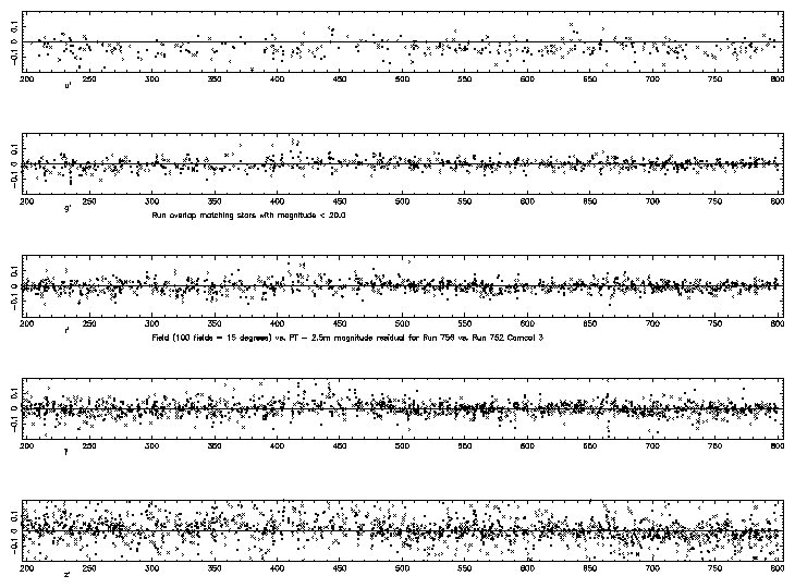
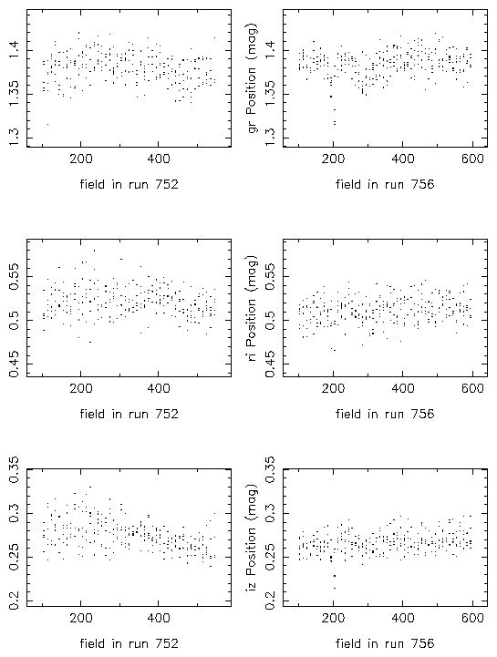
These tests consistently indicate that the photometric zeropoints for the EDR data are internally consistent to within ±2% in all bands for 90% of the frames in the EDR data. The worst outliers are all in u, and are up to 10% peak-to-peak in the worst of our data; as we saw above, these are due to ghosting in the u chip.
Because errors in different bands are often correlated, the colors of objects have smaller errors than might otherwise be indicated; stellar locii from different columns are typically aligned to better than 1% (measured in the griz bands). The median stellar locii from different runs are also aligned to better than 1%.
We discussed in § 4.4.5 that the estimated PSF magnitude errors are accurate to 10-20%. The errors themselves are impressively small, as is manifest by the width of the stellar locus; the rms scatter in bright star PSF photometry (where photon statistics are negligible), after correcting for zero-point offsets, is 0.02 mag in g*, r*, and i*, and 0.03 mag in u* and z*. The separation between the stellar locus and quasars in Figure 4.5.4 is due to this excellent photometry.
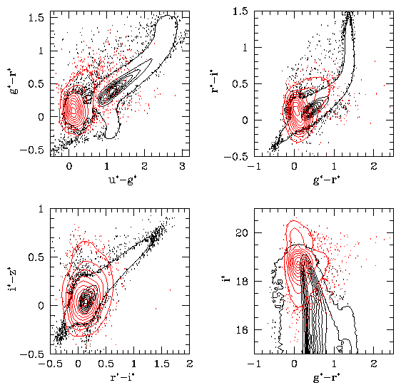
In addition to errors on the internal consistency of the photometry, the tie of the 2.5m photometry to an AB system has additional errors.
- The transfer of zeropoints from the USNO to the 2.5m
currently does not use any color terms, thereby introducing
errors in two places (USNO to PT and PT to 2.5m, as described above).
The error so introduced is of order 5%, although it may be somewhat
smaller in r, i and z.
- AB systems are based on absolute spectrophotometric measurements of standard stars, and knowledge of the broad-band response functions, as well as the overall spectrophotometric scale tied to Vega; these factors together produce uncertainties at the level of 5%.
- The zeropoints given in Fukugita et al. [1996] ignore atmospheric absorption in the bandpass shapes, introducing an error of order 4% in u and 1% in g.
Thus the system zeropoints could differ from the AB zeropoints by as much as 10%.
4.6 Imaging Data Quality Assessment
The quality of each field of data from the 2.5-meter imaging camera is assessed based on a number of criteria. A quality is assigned for each criterion, and an overall quality is assigned based on the worst value of these. The possible values for quality in the class Field (Table ) are:
- AR_DQ_GOOD: Data meet requirements
- AR_DQ_ACCEPTABLE: Data do not meet requirements but are usable for target selection; replace with new data if time permits.
- AR_DQ_HOLE: Data do not meet requirements; the area of sky is small enough to not warrant replacing with new data.
- AR_DQ_BAD: Data do not meet requirements.
- AR_DQ_MISSING: Data are missing; the area of sky is small enough to not warrant obtaining new data.
For the EDR, all fields are in one of the first three categories. The quality for each field is indicated in Figure 4.3.
A set of flags is maintained for each field in which the quality for each of the criteria is recorded. These flags are 32-bit masks; there are 4 masks, one each for GOOD, ACCEPTABLE, HOLE, and BAD, with bits assigned for each criterion used to judge quality. For example, if the seeing is judged acceptable, then the bit assigned to seeing in the ``acceptable'' mask is set. Additionally, an overall quality is stored separately.
The following are the criteria used to assess data quality:
- PSF (Seeing): The median point-spread function (PSF) full-width at half maximum (FWHM) over all 30 (photometric) CCDs must be less than 1.5 arcsec for GOOD data. Because seeing is a function of wavelength, all measures of FWHM are corrected to the value that would be measured in the r band by scaling as l-0.2. The actual algorithm also smoothes over time, so the quality of a field depends on more than just the instantaneous seeing. If the seeing fluctuates rapidly from field to field, quality is set to AR_DQ_HOLE. Additionally, for fields where the FWHM is greater than 1.5 arcsec and the largest FWHM for any CCD is less than 1.8 arcsec, the quality is AR_DQ_ACCEPTABLE.
- Tracking: The telescope must track to within 8 arcsec in the direction perpendicular to nominal path for GOOD data and 18 arcsec for ACCEPTABLE data. This is necessary to not leave gaps between adjacent scanlines.
- PSF Model: The postage stamp pipeline (§ 4.3) outputs a status flag that indicates how accurately it was able to model the variable PSF in a field. This flag is converted to a quality of GOOD, ACCEPTABLE, or HOLE.
- Timeout: For some fields, the frames pipeline requires an inordinate amount of time to process, particularly if there are complex objects such as star clusters. In such cases the pipeline processing times out and no object file is created. For such fields a HOLE is created.
- Photometric: Data must meet certain conditions on photometry. At present this quality assignment is not automated due to the complexity involved in creating a robust test. Non-photometric data are excised by hand.
- Manual: In some cases it is desirable to override the overall automated QA assignment.
The parameter badMask in Table encodes reasons why data were not declared GOOD.
The SKY and AMP bits are not used for the EDR. They are used to mask imaging data because of high sky values or bad amplifier noise, respectively.
A substantial portion of fields in the EDR have had quality set manually, overriding the PSF or tracking quality in most cases. A list of all fields that have had the quality overridden are listed in Table . They have the AR_FQ_MANUAL flag bit set.
4.7 Resolving Multiple Detections
For each stripe, 12 non-overlapping but contiguous scan lines are defined parallel to the stripe great circle. Six of these scan lines are covered when the ``north'' strip of the stripe is scanned, and the remaining six are covered by the ``south'' strip. Each scan line is 0.20977\arcdeg wide and overlaps its neighbor by approx. 1 arcmin. Each overlap region is bisected by a line of constant n. Objects in overlap regions can have a detection in each of the scan lines, and we assign one of the scan lines to have the primary detection based upon which side of the bisecting line it falls. Many queries want to consider only these objects, so we have constructed the Primary class in the catalog archive server. The classes Star, Galaxy, Sky, and Unknown are inherited from Primary. Other object detections are (usually) in the Secondary class, with its inherited classes StarSecondary, GalaxySecondary, SkySecondary, and UnknownSecondary. Two kinds of objects are not in the Primary or Secondary classes, and we put them in the Family class: objects which are tagged as BRIGHT (Table ); and parent objects which have been successfully deblended.
Object detections in the area that overlaps adjacent stripes which we have not yet observed are in the Secondary class. These may be recovered by using the status flag in Table . The flag bits AR_STATUS_OK_SCANLINE and AR_STATUS_OK_STRIPE of status are set for all objects that are within one stripe.
Objects that lie close to the bisector between scan lines present some difficulty. Errors in the centroids or astrometric calibrations can place such objects on either side of the bisector. A resolution is performed at all bisectors, and if two objects which are a primary detection lie within 2 arcsec of each other, then one object is declared primary and the other secondary.
In the EDR, most data are taken along stripes that are isolated. Runs 752 and 756 cover stripe 10, and we plan to observe the stripes adjacent to it. Therefore, only objects which do not fall in an area that will overlap with the adjacent stripes may be marked as Primary detections. Runs 94 and 125 cover stripe 82, in the southern Galactic hemisphere. We do not plan to observe the stripes adjacent to stripe 82, so all objects may be marked as Primary detections.
Objects must satisfy other criteria as well to be labeled primary; an object must not be flagged BRIGHT (as there is a duplicate ``regular'' detection of the same object; § 4.4.2), and must not be a deblended parent (as the children are already included); thus it must not be flagged BLENDED unless the NODEBLEND flag is set. These are put in the Family class.
The set of all primary detections from interleaving strips comprise a complete object catalog.
4.8 Target Selection
The spectroscopic survey aims to observe complete samples of three categories of astronomical objects (Table ):
- Galaxies, selected to be brighter than r*=17.77, using Petrosian magnitudes;
- Luminous Red Galaxies, selected by their color and magnitude to be a roughly volume-limited sample of the most luminous red ellipticals to z approx. 0.45; and
- Quasars, selected by their distinctive colors in the SDSS photometric system, and by radio detection in the FIRST survey catalog.
The following sections describe the algorithms used to select targets for spectroscopic observation. The quantity primTarget records the results of target selection for each object by using the target bit masks in Table . An object can be targeted by more than one algorithm. The quasar and galaxy targets are marked as ``tiled'' in the table to indicate that we intend to obtain a uniform and complete sample. The TARGET_STAR_BROWN_DWARF and TARGET_HOT_STD targets are also tiled, as described below.
The data included in the EDR are commissioning data, and were used, among other things, to refine the algorithms discussed here. Table lists the versions of the target pipeline that were used to select which objects to observe spectroscopically. The exact algorithms used are not uniform throughout all the data released, and Table summarizes the important differences. The results of target selection are recorded in the quantity PrimTarget, which appears in two classes. The class SpecObj records the results of target we used to select objects for spectroscopic observation (v2.2a, v2.5, and v2.7), while the class PhotoObj records the results of target run on the final photometric catalog (target v2.13.8).
The galaxy magnitude limit has changed slightly, as has the criterion for selecting low-surface brightness galaxies, and a number of changes have been made to quasar target selection. Since the pipeline software versions, the photometric calibration, and target selection criteria change, there will be slight mis-matches between the value of PrimTarget for the same object recorded in class SpecObj and PhotoObj.
The quasar selection algorithm is substantially different in target v2.13.8. A complete description of these improvements is beyond the scope of this paper.
4.8.1 Galaxies
Images of galaxies are distinguished from images of stars by morphology. As described above (§ 4.4.6), we separate stars from galaxies using the difference between the PSF and model magnitude in r*. Galaxy target selection requires a difference greater than 0.3 mag. During commissioning, we changed the magnitude limit of the sample several times (Table ), and experimented with a fuzzy limit, whereby the probability that a galaxy be selected was a declining function of r* over a range of 0.1 magnitudes. For the EDR, a sharp magnitude cut of r*Petrosian = 17.5 yields a complete sample of galaxies, with a surface density of order 90 galaxies per square degree (see the discussion in § 4.9).
All magnitudes are corrected for extinction following Schlegel, Finkbeiner, & Davis [1998]. Objects with fiber magnitudes brighter than 15 in g* or r*, or brighter than 14.5 in i* are rejected, to avoid problems with fiber cross-talk in the spectrographs, for target v2.7, runs 94 and 125, as indicated in Table . We also reject objects with SATUR set, which unfortunately rejects galaxies blended with saturated stars. Finally, the more recent versions of target reject objects with PetroR50 < 2˘˘, brighter than r* = 15.5 (v2.7) and 15.0 (v2.13.8), to cut down on contamination from very bright stars.
We have found that galaxy targets of very low surface brightness are often not real objects, but are due to very low-level scattered light within the camera. We therefore put in an explicit surface brightness cut. A Petrosian half-light surface brightness is defined as the mean surface brightness within the radius, PetroR50, which includes half the Petrosian flux. All objects with Petrosian surface brightness fainter than the value listed in Table are not targeted (the surface brightness limit of 30.0 for v2.5 indicates that in effect, no surface brightness cut was applied).
For target v2.13.8, we check that for faint objects, the local sky value in r is sensible. Objects with surface brightness between 23.0 and 24.5 are only selected if the value of the sky determined locally (i.e., on scales of ~ 2 arcmin, sky in class PhotoObj) and that on a frame (10 arcmin scales, sky in class Field) are within 0.05 asinh mag per square arcsec of one another; the local sky of a child includes the contribution of its siblings, so this cut discriminates against pieces of fluff inadvertently deblended from bright galaxies. These objects are flagged both TARGET_GALAXY and TARGET_GALAXY_BIG.
Finally, galaxies with fiber magnitude brighter than r* = 19 that don't otherwise make the surface brightness cut are targeted. These are flagged TARGET_GALAXY_BRIGHT_CORE. Such objects are quite rare.
The resulting sample is contaminated at the approx. 1% level by close double stars that are not separated by the deblender. The details of the galaxy target selection, and the tests to show that it works, are described in Strauss et al. [2001].
4.8.2 Luminous Red Galaxies
It has long been known that the most luminous galaxies in clusters are a very homogeneous population (e.g., Postman & Lauer 1995 and references therein); they have a very narrow range of color and intrinsic luminosity. Because these objects are intrinsically very luminous, they can be observed to great distance.
We therefore selected such objects by a variant of the method of
photometric redshifts (), with the aim of selecting
a uniform, approximately volume-limited sample of objects with the
reddest colors in the rest frame [Eisenstein et al., 2001]. We term these
objects ``Luminous Red Galaxies'', or LRGs.
It turns out that this can be
simply done with cuts in the g*-r*, r*-i*, r*
color-color-magnitude cube. Because the 4000Å break
moves from the g band to the r band at zapprox. 0.4, two
different sets of selection criteria are used, which we term Cut I and
Cut II. First, we rotate to a
color basis that is aligned with the galaxy locus in the g*-r*,
r*-i* plane as follows:
|
Cut I and Cut II objects used star-galaxy separation criteria that
changed from one chunk to another (Table ).
For Cut I, the flux and color cuts are:
|
This gives an approximately volume-limited sample of galaxies to z = 0.37 with additional galaxies up to zapprox. 0.45. These objects are flagged GALAXY_RED.
To reach higher redshifts, we use Cut II:
|
The luminosity cut in Cut I (eq. [17]) is a good approximation to a passively-evolving old stellar population from zapprox. 0.15 to zapprox. 0.45, but is too permissive at lower redshift. At z < 0.20, one should not use the GALAXY_RED flag to extract the low-redshift extension of the LRG volume-limited sample. Rather, one must use the redshift extracted from the main galaxy sample to construct the absolute magnitude and rest-frame color and select galaxies that fall in the region populated by the high-redshift LRGs. This is described in more detail in Eisenstein et al. [2001].
The resulting LRG sample has nearly constant comoving number density to zapprox. 0.4 with a passively-evolved luminosity threshold that is close to constant. This suggests that the sample is indeed close to the volume-limited goal. At z > 0.4, the sample is effectively flux-limited but still selects intrinsically red galaxies. The sample selection is also quite efficient: 97% of the selected targets are at z > 0.15.
The two LRG Cuts together give roughly 12 targets per square degree that are not already in the main galaxy target selection sample, typically 10 of which are Cut I targets and 2 of which are Cut II targets.
4.8.3 Quasars
Images of quasars are characterized in the optical by high luminosity and very high surface brightness, making them morphologically indistinguishable from stars at all but very low redshifts (z Ł 0.6 at the resolution of the SDSS). Quasar spectra, however, are characterized by roughly power-law continua and strong emission lines; as a result, quasar spectra are quite distinct from the roughly black-body spectra of stars.
The dominance of the continuum on the colors of quasars is severely reduced because of absorption by the Lya forest and Lyman-limit systems (at rest wavelengths below 1216 Å and 912 Å, respectively). For the SDSS filter set, absorption by the Lya forest is significant for z ł 2.2, and quasars become increasingly red with larger redshift [Fan, 1999,Richards et al., 2001a]. Fortunately, this effect also gives quasars colors that are distinctly different from those of normal stars.
Models of quasars by Fan [1999] show that the quasar locus is indeed well-separated from the stellar locus except at z = 2.7-2.8, where quasars have SDSS broad-band colors that are essentially indistinguishable from early F and late A stars. Thus the majority of quasars have colors quite distinct from those of stars, which, unlike quasars, lie on a nearly one-dimensional locus in (u*-g*),(g*-r*),(r*-i*),(i*-z*) color-color-color-color space [Newberg & Yanny, 1997,Fan, 1999,Finlator et al., 2000]. Using this property, we identify quasar candidates primarily as outliers from the stellar locus in this 4-color space. This algorithm is described in more detail by Richards et al. [2001b].
The quasar target selection algorithm first models the stellar locus, following Newberg & Yanny [1997], as an elongated tube with an elliptical cross-section. In practice, this is done in two stages, once for the (u*-g*), (g*-r*), (r*-i*) color cube, and once for the (g*-r*),(r*-i*), (i*-z*) color cube. The PSF colors of each object are examined in turn, and it is determined whether they are consistent with lying inside the stellar locus, incorporating the photometric errors. The quoted errors in PSF magnitudes from frames are used, after adding approx. 0.03 mag errors in quadrature in each color to reflect the uncertainty in the photometric calibration. Quasar candidates are those objects which lie more than 4 s from the stellar locus. Colors are measured using PSF magnitudes, and are corrected for reddening using Schlegel, Finkbeiner, & Davis [1998] throughout.
The quantity objFlags in class photoObj uses the bitmasks in Table to indicate objects whose photometry (and therefore, colors) may be in error. In particular, we reject objects flagged as BLENDED (although we accept the deblended children of blended parents), BRIGHT, SATURATED, or EDGE in any band. Objects detected as MOVING at a rate greater than 0.2 pixels per frame with high significance are rejected as asteroids (although this rejection is no longer needed in the current algorithm; asteroids have colors that put them cleanly in the stellar locus; ). Deblended children with PEAKCENTER, NOTCHECKED, or DEBLEND_NOPEAK set in any band are signs of deblending problems; these objects are also rejected. Objects with INTERP_CENTER set have a cosmic ray or bad column within 3 pixels of their center; empirically, we find that many false quasar candidates are found with i* < 16.5 and this flag set, so we reject all such objects. There are a few bad columns which are not properly interpolated over by the photometric pipeline, and so we reject objects in CCD columns 1019-1031 in camCol 5.
At one point, we had considered separate criteria in regions of high and low stellar density, as we were concerned about changing stellar populations at low latitudes. For this reason, objects that pass the main quasar target selection criteria have the TARGET_QSO_CAP (referring to the Galactic cap) or TARGET_QSO_SKIRT (the ring around Galactic cap region), target mask bit set in primTarget of class specObj, depending on their Galactic coordinates and, in particular, the estimated stellar density from the Bahcall & Soneira [1980] model. However, we found that the effectiveness of the algorithm was independent of stellar density, so the selection of the two is identical.
An outlier from the (u*-g*), (g*-r*), (r*-i*) color cube is a quasar candidate if it passes the above gauntlet of tests and has 15.0 < i* < 19.0. The bright limit is set to avoid problems with cross-talk in the spectrographs. As indicated in Table , the bright limit used for target version v2.2.a, runs 752 and 756 was i* = 16.5. The object need not be stellar if it lies blueward of the main galaxy locus; this allows low-redshift AGN, whose host galaxy is visible, to be selected.
We reject some quasar candidates if they have colors that match known types of
stars which lie outside the main stellar locus. In particular, hot
white dwarfs are excluded when
,,
| (21) |
| (22) |
| (23) |
The quasar locus crosses the stellar locus for quasars of z ~ 2.7, so
we include target objects when
,
| (24) |
Each of these three regimes of stars were rejected in the EDR data (as indicated in Table ), except with target version v2.2a, runs 752 and 756, when only the A star rejection was applied. Inclusion of objects in the region where the stellar and quasar loci cross was performed for all three versions of target used for the EDR.
The SDSS catalog is matched against the FIRST catalog of radio sources [Becker, White, & Helfand, 1995], and stellar objects with radio counterparts within 2\arcsec and i* < 19.0 are selected, using the mask bit TARGET_QSO_FIRST_CAP or TARGET_QSO_FIRST_SKIRT depending on their position on the sky.
The mask bit in primTarget we use for the high redshift quasar sample is TARGET_QSO_HIZ. Outliers from the stellar locus in the (g*-r*), (r*-i*), (i*-z*) color cube with i* < 20.0 are selected, subject to the rejection criteria given above in equations 20, 21, and 22. Additionally, candidates must be classified as stellar, as they will have redshifts above z = 3.5 for the most part (see the discussion in Fan et al. 2001a). For target versions v2.5 and v2.7, we also targeted objects which lie in the region of color-color space for z > 3, are still outliers in the (u*-g*), (g*-r*), (r*-i*) cube and have u*-g* > 1.5 and i* < 20.0, see Table .
Although low-redshift quasars manifest themselves most dramatically as
outliers in u*-g*, they are also outliers in the g*r*i*z* color
cube, and would thus dominate the (nominally) high-redshift color cut, which
goes fainter than the main quasar sample. Therefore, we rejected very blue
objects that satisfy
,,
|
For target versions v2.2.a, v2.5, and v2.7, objects which lie outside the stellar locus, but are fainter than the magnitude limit, are flagged as TARGET_QSO_FAINT; they are not targeted, but are marked as being of potential interest. We emphasize, however, that the algorithm is not optimized fainter than i*=20.0, so the fraction of objects flagged as TARGET_QSO_FAINT that turn out to be quasars will decrease significantly with magnitude. Objects with this flag set will only have spectra if they were targeted by another module.
Quasar candidates are selected primarily as objects with colors distinct from stars, allowing the serendipitous discovery of a variety of objects of unusual color, including those that do not conform to ``standard'' quasar colors. It has thus found a number of very unusual BAL quasars, extreme emission-line galaxies, high-redshift (z > 0.7) starburst and post-starburst galaxies, and a handful of objects whose spectra defy classification.
This algorithm selects of order 15 objects per square degree. Our target efficiency requirement is that at least 65% of our quasar candidates should in fact be quasars. The EDR is very close to meeting this requirement, and we certainly expect future data releases to meet or exceed this requirement. The principal contaminants are compact blue star-forming galaxies at low redshift; A stars; white dwarfs and M dwarf-white dwarf pairs that the above color cuts don't completely remove; and a variety of exotica such as z > 0.4 compact E+A galaxies, whose Balmer break gives them colors very similar to z=4 quasars. Comparison with quasars from the literature shows that our completeness is of order 90%, which is consistent with our completeness requirement. Known quasars that are not targeted are rejected for a wide variety of reasons: many are due to cosmetic defects, and many z=3.5 and z=4.5 quasars are missing due to problems with the quasar target selection code, which have been corrected since target was run to define the plates in the EDR.
4.8.4 Other Science Targets
A variety of other science targets are selected. These include optical counterparts of ROSAT sources, stars, and serendipitous targets. These samples are not complete (with the exception of spectrophotometric standards and brown dwarfs), but are assigned to excess fibers left over after the main samples of galaxies, LRG's, and quasars are tiled (§ 4.9).
For typical values of the ratio of optical to X-ray flux of various classes of Galactic and extragalactic sources, there is an excellent match between the depth of SDSS in the optical and that of the ROSAT All Sky Survey (RASS; ) in X-rays. Objects detected in SDSS imaging data are positionally matched against X-ray sources from the RASS catalogs. SDSS objects within the RASS positional error circles (commonly 10-20˘˘ radius) are scrutinized further by target selection algorithms tuned to select likely optical counterparts to the X-ray sources. In decreasing priority order, spectra are obtained for SDSS/RASS coincidences that: (a) are also radio sources (flagged ROSAT_A); (b) have SDSS optical colors of AGN/quasars (ROSAT_B); (c) fall in a broad intermediate priority bin that includes bright and/or moderately blue stars and galaxies (ROSAT_C); (d) are otherwise bright enough for follow-up spectroscopy (ROSAT_D). Objects flagged ROSAT_E are not targeted; they fall within the ROSAT error circle, but are either too faint or too bright for our spectrographs. Objects with fiber magnitude brighter than 15 in g*, r*, or i* are not targeted, because of cross-talk between fibers in the spectrograph.
This algorithm targets of order 10-15 objects per plate; over half are AGN or quasars.
A variety of stars are also targeted by their distinctive colors. Specific stellar spectroscopic target categories include blue horizontal branch stars (flagged STAR_BHB), carbon stars, both dwarf and giant ( STAR_CARBON), low-luminosity subdwarfs (STAR_SUB_DWARF), the central stars of planetary nebulae (STAR_PN), cataclysmic variables (CATY_VAR), red and brown dwarfs (STAR_RED_DWARF and STAR_BROWN_DWARF), and hot white dwarfs (STAR_WHITE_DWARF). The planetary nebula and cataclysmic variable categories are essentially completely contained within the quasar target selection region of color-color space, and are much rarer than quasars; only a handful of these objects have been found. The definition of red dwarf was too inclusive in the version of target used, resulting in the observations of a large number of ordinary M dwarfs. The brown dwarfs are very rare (typically one every several plates); unlike the other categories of stars, these are tiled. However, in the EDR data, the algorithm for selecting these objects was modified several times, making the formal definition of a complete sample difficult.
Additionally, of order 30% of the objects targeted as quasars turn out, in fact, to be stars, for the most part outliers from the stellar locus by definition (but occasionally objects in the stellar locus as well, due to early errors in the code). This is of course not a complete sample, but it contains several thousand spectra of uniform data quality of stars of all spectral types.
Finally, we have an open category of targets, referred to as serendipity, whose criteria are subject to change as different regions of parameter space are explored. There are several categories of these in the EDR. These are flagged as SERENDIP_RED, SERENDIP_BLUE, and SERENDIP_DISTANT for objects lying outside the stellar locus in color space (the latter refers to distance from the stellar locus). These overlap somewhat with the quasar and some of the stellar target selection categories. Objects coincident with FIRST radio sources are flagged SERENDIP_FIRST; this matching goes fainter than the equivalent for quasar target selection, and has no restriction on stellarity. Finally, SERENDIP_MANUAL targets are selected by hand, as the name implies. A wide variety of interesting objects have emerged from serendipity spectroscopic targets, ranging from highly unusual categories of white dwarfs to radio-loud broad absorption line quasars [Menou et al., 2001].
4.8.5 Calibration Targets
In addition to science targets, about 50 fibers out of each plate of 640 are assigned by target for calibration spectra. Since spectroscopy requires good sky subtraction, 32 of these calibration fibers are assigned to regions where the photometric pipeline detects no objects (in fact, the photometric pipeline outputs several such ``sky objects'' in each frame for this purpose). These sky fibers are distributed so that each bundle of 20 fibers contains one; this ensures that the sky fibers are reasonably uniformly distributed around the plate. In addition, 18 fibers per plate are assigned to standard stars of various sorts; eight are spectrophotometric standards, chosen to be F dwarfs, eight are reddening standards, chosen to be F subdwarfs, and two are hot subdwarfs (Table ). The spectrophotometric standards are also used in correcting the strong telluric water absorption bands in the red end of the science target spectra (the smoothness of the F subdwarf spectra make them ideal for this purpose). Conversely, the hot subdwarfs are useful for calibrating the blue end of the science target spectra. Finally, as their name implies, the reddening standards will be used for determining the reddening of our Galaxy.
Further details of the spectroscopic calibration process are discussed in § 4.10.1.
4.8.6 Target Culling
In regions of particularly poor seeing, the colors of stars were occasionally systematically off, especially when earlier versions of photo were used. This caused the target selection algorithms that select outliers in color-color space to choose an inordinate number of targets. We corrected for this by manually culling targets from the list.
In particular, target candidates were culled from run 752 (Target v2.2a) in 61 fields due to problems caused by poor seeing. In fields with 5 or more quasar candidates, we removed candidates which were not also selected as galaxy targets, in the following categories:
- TARGET_QSO_HIZ, TARGET_QSO_CAP, TARGET_QSO_SKIRT,
- TARGET_QSO_FIRST_CAP, TARGET_QSO_FIRST_SKIRT,
- TARGET_SERENDIP_BLUE, TARGET_SERENDIP_RED,
- TARGET_SERENDIP_DISTANT, TARGET_STAR_SUB_DWARF,
- TARGET_STAR_WHITE_DWARF, TARGET_STAR_CARBON.
Similarly, target candidates in runs 94, 125 (Target v2.7) were culled from 52 fields. Additionally, all QSO_HIZ candidates in run 94 in camera column 6 were removed from the list. This was necessary due to a problem with the characterization of the point spread function in the version of the psp used at the time.
After the plates from run 94/125 were drilled, we discovered that many quasar candidates were targeted, due to an error in the target selection code. Spectra were collected for these targets, but they may be removed from quasar analyses by rejecting objects which satisfy the criterion: ,( 0.65 < u*-g* < 0.9) (0.2 < g*-r* < 0.9).
4.9 Plate Definition
Once target selection has been completed, the spectroscopic plates need to be positioned and fibers assigned to targets. As noted above, although each plate can accommodate 640 fibers, about 50 of these are reserved for calibration targets, leaving around 590 fibers for science targets; for plates 266-315 the available number was 588 and for later plates the number was 592. As described in this section and in Table , a number of object types are potential spectroscopic science targets. However, only for some of these do we attempt to obtain a uniform and complete sample, the so-called ``tiled targets,'' as indicated in Table . Other science targets, such as most types of stars, ROSAT sources, serendipity targets, etc., are assigned leftover fibers according to a set of priorities after the plates are positioned and fibers are assigned to tiled targets.
To position the plates, we could simply place them on a uniform grid, but given the clustering of the galaxy targets which dominate the sample, this procedure would give some plates substantially more targets than available fibers, while others would have large numbers of extra fibers. To make best use of observing time, an algorithm based on cost-minimization [Blanton et al., 2001b] determines the optimal positioning of plate centers in order to maximize the number of tiled targets on which a fiber can be placed. This spaces plates more closely together in regions with a larger density of galaxies, increasing the completeness and efficiency of the spectroscopic survey. This process of optimally placing spectroscopic plates is referred to as tiling.
Due to the finite diameter of the fibers and their cladding, fibers cannot be placed more closely than 55 arcsec from one another. For each group of targets within 55˘˘, we put fibers on the largest possible set of the highest priority objects; in case there is a tie, we decide on the competing configurations based on the next highest priority objects, and so on. Brown dwarf and hot standard star targets have priority over quasar targets, which have priority over luminous red galaxies and main sample galaxies. The priorities of each object are stored in a parameter priority; a higher value means higher priority. This procedure means that if two objects of the same priority are within 55˘˘, one is rejected at random. Roughly 8-9% of targeted objects are not targeted for this reason, in regions covered by a single plate. In regions of plate overlap, of course, both objects in such a close pair can be targeted; about 30% of the sky is covered by such overlaps. Finally, there is another constraint, which is that no fiber can be placed within 100˘˘ of the center of a plate; this excludes a very small number of targets.
Due to an error in an early version of the tiling pipeline, for the earliest plates (266-315) three gaps were left in the assignment of fibers to tiled targets. Because of the nature of the bug, these occurred in regions where plates overlapped; also, they unfortunately tended to occur in the densest regions. They occurred in the overlaps between plates 270 and 271, plates 312 and 313, and plates 314 and 315.
The bookkeeping of the tiling results has not been provided in this data release, including whether a fiber was eliminated due to a collision and whether it was originally targeted in the ``drilling'' version of the data reductions. Future data releases will include this information. However, it is possible to evaluate the completeness from the data itself by calculating the fraction of each target type (as determined in the released version of the reductions) which have spectra; simply be careful to include the effect of fiber collisions. We have determined that for South Equatorial Stripe and the SIRTF First Look Field, the effective flux limit for the main galaxy sample is about r*=17.5; for the North Equatorial Stripe, the effective flux limit is about r*=17.6. Finally, because there may be incompleteness in regions covered by one observed plate and one unobserved plate, it is important to know the locations of the unobserved plates when evaluating the window function of the survey. Thus, we include in Table the locations of plates not released here.
As discussed above in § 4.8.6, we found that target selection did poorly in a few regions of sky of particularly bad seeing, especially with earlier versions of the imaging pipelines. The symptom was typically an excessive number of quasar candidates due to poor photometry. We were forced in a few regions therefore to cull the spectroscopic targets.
4.10 Spectroscopic Pipelines
The spectroscopic pipelines, spectro2d and spectro1d, reduce the two-dimensional spectrograms produced by the spectrographs to flux- and wavelength-calibrated spectra, and then measure emission and absorption features, classify the spectra, and measure redshifts.
The spectro2d pipeline reduces the raw data and calibration images from the red and blue CCD cameras from each spectrograph and produces merged, co-added, calibrated spectra, noise estimates, and mask arrays (see Table ) for analysis by the spectro1d pipeline. All wavelengths are expressed in Å, and are vacuum wavelengths corrected to the heliocentric frame, while the flux density fl is in units of 10-17 erg cm-2 s-1 Å-1.
The spectro1d pipeline determines emission and absorption redshifts, classifies spectra by object type, and measure lines in each spectrum. The class specObj (Table ) contains parameters measured for the entire spectrum, as well as links to the Plate that the spectrum is from, the PhotoObj information for the object, and links to objects in Table : SpecLine, lines identified and measured; SpecLineName, names for the lines; SpecLineIndex, equivalent widths and redshifts; CrossCorrelationRedshift, measures of the cross correlation redshift; and EmissionRedshift, measures of the emission redshifts.
We also provide the flux- and wavelength-calibrated spectrum, the spectrum with continuum subtracted, and the estimate of the 1 s error per pixel, all in the units above, plus the mask array, as described in § 2.5.
4.10.1 Extraction and Calibration of Spectra
The spectro2d pipeline works in two stages. First, it reduces the data from each chip from each fifteen-minute exposure separately, and then it combines the results from each exposure.
After bias subtraction, each raw image is divided by a uniformly illuminated flat to take out pixel-to-pixel variations. The flat-field spectra (i.e., the flat-field observed through the fibers) are then traced on the CCD: for each fiber, the flat-field image centroid in column position is fit by a polynomial in row number. The flat-field spectra are optimally extracted, assuming a Gaussian profile for each one, simultaneously fitting a low-order polynomial to scattered light. These fits will also be used for the first-order object extraction of the science and arc frames, allowing for small offsets. The arc lamp spectra are extracted as well and centroids of the lines are measured, to which we fit a fifth-order Legendre polynomial.
The flat-field spectra are then wavelength-calibrated, normalized, and combined to form a ``superflat'' for each spectrograph camera, by stacking the 320 normalized flat-field spectra and performing an iterative least-squares bspline fit with outlier rejection on this 320 ×2048 oversampled dataset to obtain an effectively continuous function. For each fiber, the superflat is resampled at every pixel and divided into the extracted flat-field spectrum to form the ``fiber flat.'' In this way, flat-field variations between fibers are removed, as are small-scale features in the wavelength dependence of the system response.
For the science exposures, the object and sky fibers are spatially traced, with tweaking from the flat-field trace, and optimally extracted. In the extraction, the Gaussian fiber profile fitting can also be tweaked from the fiber-flat image. Scattered light is removed by a fourth order Chebyshev polynomial fit. Outlying pixels are rejected and masked. The extracted spectra are then flat-fielded by dividing by the fiber flats, and the wavelength solution is applied, using a vacuum wavelength scale, adjusting slightly to match the known positions of certain sky lines, and correcting to the heliocentric frame. The wavelength calibration is accurate to of order 10 km s-1 or better.
As with the flats, an oversampled ``supersky'' is constructed from the 32 sky fibers per plate. For each fiber, the supersky is resampled at every pixel in the object spectrum and subtracted.
Telluric absorption in four wavelength regions in the red spectra is removed using spectrophotometric and reddening standard stars: these are used to construct four ``superTelluric'' spectra using the bspline fitting procedure.
Next, spectro2d performs a spectrophotometric flux calibration of the individual exposures: the counts in each exposure are placed on the same scale, and the wavelength scale is rebinned to a simple polynomial in log l.
If a smear exposure exists, the counts in each exposure are corrected to match a low-order fit to the smear counts; this corrects for light which falls outside the 3˘˘ fiber aperture because of seeing, guiding errors, and atmospheric refraction. However, since the smear exposure procedure was implemented part way through commissioning, many of the plates included in the EDR do not have smear exposures (see Table ).
Next, the spectra are flux-calibrated by matching the counts in the mean of the high S/N spectra of the spectrophotometric and reddening standards on the plate, and equating this to the synthetic composite F8 subdwarf spectrum from Pickles (1998). This is placed on an absolute scale by matching the synthesized r* fiber magnitudes of these stars to the SDSS photometry14. This procedure removes the instrument response as a function of wavelength in each spectrograph camera. The absolute accuracy of the spectrophotometry is not well-measured at this point, but can probably be trusted to 20% for point sources when smear exposures are available. Note that for extended sources (galaxies), the smear technique effectively corrects the spectrophotometry to a 5˘˘×8˘˘ aperture; in the presence of spectral gradients (e.g., nuclear emission lines), the results may be difficult to interpret.
Finally, for each object, the individual science frames, both red and blue halves, are stacked and fit with the iterative bspline, with inverse variance weighting. In the process, outliers due to cosmic rays are rejected and masked, and errors in the fluxes estimated. The combined, merged spectra are resampled in constant velocity pixels (logl), with a pixel scale of 69 km sec-1. If possible, exposures on multiple nights are combined. If a plate is re-plugged, however, only the exposures with a given plugging are combined.
Mask bits are set for each pixel of the reduced spectra, as described in Table . Two masks are given for the final combined spectra, the bits in the OR mask set if the relevant flag was set in any of the individual exposures entering the combination, while the AND mask indicates that the flag was set in all of the exposures for that pixel. For most purposes, one should examine the OR mask to be safe. Pixels flagged FULLREJECT, NOSKY, NODATA, or BRIGHTSKY, or those with error set to identically zero are likely to be corrupted. Many of these are due to bad columns on the CCD's, or cross-talk from very bright objects in neighboring fibers (see the flag NEARWHOPPER).
On occasion, the spectra exhibit unphysical wiggles due to problems in the spectrophotometry, especially in the region of the dichroic split ( ~ 6000Å); this will be improved in future releases.
4.10.2 Measuring Spectra
The spectro1d pipeline analyzes the combined, merged spectra output by spectro2d and determines object classifications (galaxy, quasar, star, or unknown) and redshifts; it also provides various line measurements and warning flags.
The code attempts to measure an emission and absorption redshift independently for every targeted (non-sky) object. That is, to avoid biases, the absorption and emission codes operate independently, and they both operate independently of any target selection information.
The spectro1d pipeline performs a sequence of tasks for each object spectrum on a plate: The spectrum and error array are read in, along with the pixel mask. Pixels with mask bits set to FULLREJECT, NOSKY, NODATA, or BRIGHTSKY are given no weight in the spectro1d routines. The continuum is then fit with a 5th order polynomial, with iterative rejection of outliers (e.g., strong lines). The fit continuum is subtracted from the spectrum. The continuum-subtracted spectra are used for cross-correlating with the stellar templates.
Emission lines (peaks in the 1d spectrum) are found by carrying out a
wavelet transform of the
continuum-subtracted spectrum fc(l):
| (26) |
This list of lines with non-zero weights is matched against a list of common galaxy and quasar emission lines given in Table , many of which were measured from the composite quasar spectrum of Vanden Berk et al. [2001] (due to velocity shifts of different lines in quasars, the wavelengths listed don't necessarily match their rest-frame values). Each significant peak found by the wavelet routine is assigned a trial line identification from the common list (e.g., ) and an associated trial redshift. The peak is fit with a Gaussian, and the line center, width, and height above the continuum are stored in the SpecLine class as parameters wave, sigma, and height, respectively. If the code detects close neighboring lines, it fits them with multiple Gaussians. Depending on the trial line identification, the linewidth it tries to fit is physically constrained. The code then searches for the other expected common emission lines at the appropriate wavelengths for that trial redshift and computes a Confidence Level (CL) by summing over the weights of the found lines and dividing by the summed weights of the expected lines. The CL is penalized if the different line centers do not quite match. Once all the trial line identifications/redshifts have been explored, an emission line redshift is chosen as the one with the highest CL, and stored as z in the EmissionRedshift class. The exact expression for the emission line CL has been tweaked to match our empirical success rate in assigning correct emission line redshifts, based on manual inspection of a large number of spectra from the EDR (§ 4.10.3).
The SpecLine class also gives the errors, continuum, equivalent width, c2, spectral index, and significance of each line, in parameters listed in Table . We caution that the emission line measurement for Ha should only be used if c2dof < 2.5. In the SpecLine class, ``found'' lines denote only those lines used to measure the emission line redshift, while ``measured'' lines are all lines in the emission line list (Table ) measured at the redshifted positions appropriate to the final redshift assigned to the object.
A separate routine searches for high-redshift (z > 2.3) quasars by identifying spectra that contain a Lya forest signature: a broad emission line with more fluctuation on the blue side than on the red side of the line. The routine outputs the wavelength of the Lya emission line; while this allows a determination of the redshift, it is not a high-precision estimate, because the Lya line is intrinsically broad and affected by Lya absorption. The spectro1d pipeline stores this as an additional emission-line redshift. This redshift information is stored in the EmissionRedshift class (Table ), which includes an association to an object in the SpecObj class. Thus one SpecObj can have one or two EmissionRedshift objects associated with it.
If the highest CL emission line redshift uses lines only expected for quasars (e.g., Lya, , ]; see Table ), then the object is provisionally classified as a quasar. If any of the identified lines is broader than 500 km sec-1 (FWHM), then the object is also provisionally classified as a quasar for the EDR. We expect that this threshold will change in future data releases. These provisional classifications will hold up if the final redshift assigned to the object (see below) agrees with its emission redshift.
The spectra are cross-correlated with stellar, emission-line galaxy, and quasar template spectra to determine a cross-correlation redshift and error. The cross-correlation templates are obtained from SDSS commissioning spectra of high S/N, and comprise roughly one for each stellar spectral type from B to almost L, a non-magnetic and a magnetic white dwarf, an emission line galaxy, a composite LRG spectrum, and a composite quasar spectrum (from ). The composites are based on co-additions of ~ 2000 spectra each. The template redshifts are determined by cross-correlation with a large number of stellar spectra from SDSS observations of the M67 star cluster, whose radial velocity is precisely known.
When an object spectrum is cross-correlated with the stellar templates, its found emission lines are masked out; i.e., the redshift is derived from the absorption features. The cross-correlation routine follows the technique of Tonry & Davis [1979]: the continuum-subtracted spectrum is Fourier-transformed and convolved with the transform of each template. For each template, the three highest Cross-Correlation Function (CCF) peaks are found, fit with parabolas, and output with their associated confidence limits (CLs). The corresponding redshift errors are given by the widths of the CCF peaks. The cross-correlation CLs are empirically calibrated as a function of peak level based on manual inspection of a large number of spectra from the EDR. The final cross-correlation redshift is then chosen as the one with the highest CL from among all the templates.
If there are discrepant high-CL cross-correlation peaks, i.e., if the highest peak has CL < 0.99 and the next highest peak corresponds to a CL that is greater than 70% of the highest peak, then the code extends the cross-correlation analysis for the corresponding templates to lower wavenumber and includes the continuum in the analysis, i.e., it chooses the redshift based on which template provides a better match to the continuum shape of the object. These flagged spectra are then manually inspected (see below).
The cross-correlation redshift is stored as z in the CrossCorrelationRedshift class.
The spectro1d pipeline assigns a final redshift to each object spectrum by choosing the emission or cross-correlation redshift with the highest CL, and stores this as z in the SpecObj class. A redshift status bitmask (zStatus) and a redshift warning bitmask ( zWarning) are stored, with bitmask values given in Table . The CL is stored in zConf. Objects with redshifts determined manually (see below) have CL set to 0.95 (MANUAL_HIC set in zStatus ), or 0.4 or 0.65 (both MANUAL_LOC set in zStatus). Rarely, objects have the entire red or blue half of the spectrum missing; such objects have their CLs reduced by a factor of 2, so they are automatically flagged as having low confidence, and the mask bits Z_WARNING_NO_BLUE or Z_WARNING_NO_RED are set in zWarning as appropriate.
All objects are classified (in specClass) as either a quasar, high-z quasar, galaxy, star, late-type star, or unknown. If the object has been identified as a quasar by the emission line routine, and if the emission line redshift is chosen as the final redshift, then the object retains its quasar classification. Also, if the quasar cross-correlation template provides the final redshift for the object, then the object is classified as a quasar. If the object has a final redshift z > 2.3 (so that Lya is or should be present in the spectrum), and if at least 2 out of 3 redshift estimators agree on this (the 3 estimators being the emission-line, Lya, and cross-correlation redshifts), then it is classified as a high-z quasar. If the object has a redshift cz < 450 km sec-1, then it is classified as a star. If the final redshift is obtained from one of the late-type stellar cross-correlation templates, it is classified as a late-type star. If the object has a cross-correlation CL < 0.25, it is classified as unknown.
There exist among the spectra a small number of composite objects. Most common are bright stars on top of galaxies, but there are also galaxy-galaxy pairs at distinct redshifts, and at least one galaxy-quasar pair, and one galaxy-star pair. Most of these have the zWarning flag set, indicating that more than one redshift was found.
For all objects, Gaussians are fit at the positions of all expected emission lines in the reference list (see Table ), not just the common lines, and their parameters are stored in the class SpecLineIndex (Table ).
For galaxies, we compute in the rest frame: the equivalent width, magnitude, and their errors of a number of standard line indices, which are useful for stellar population, age, and metallicity measures. These are stored in ew, ewErr, mag, and magErr in the class SpecLineIndex. The equivalent width and magnitude are not corrected for velocity dispersion. We only recommend the use of these line indices for stellar population studies for galaxy spectra with good signal to noise ratio: sn[0] of class SpecObj should be greater than 30.
A complete list of the lines we measure is available on our web sites. They were gathered from the following sources:
- Lick line indices (21 absorption-line strengths on the revised Lick/IDS line-strength system) [Trager et al., 1998]
- CN, H+K, , G, Hb, Mg, MH, FC, NaD [Brodie & Hanes, 1986]
- 8498, 8542, 8662, 8807 [Diaz, Terlevich, & Terlevich, 1989].
We also calculate a measure of the strength of the 4000Å break as the ratio of the flux from 3751-3951Å to the flux from 4051-4251Å, and the ratio of the strength of the Ca K and H lines, as integrated from 3921-3946Å and 3956-3981Å, respectively. These are also stored as ``lines'' in the class SpecLineIndex, with the flux ratio stored in the parameter ew. This flux ratio is used as a sanity check on the spectra. If the break is in the wrong direction (flux decreasing with increasing l), or if the flux ratio is greater than 0.95, the Z_WARNING_4000BREAK bit is set in zWarning.
Finally, galaxies are classified by a Principal Component Analysis (PCA) (, as extended by ), using cross-correlation with eigentemplates constructed from early SDSS spectroscopic data. The 5 eigencoefficients and a classification number are stored in eCoeff and eClass, respectively, in the SpecObj class. eClass ranges from about -0.35 to 0.5 for early- to late-type galaxies.
In future data releases, we expect to implement more detailed stellar spectral classification based on a larger set of stellar templates. The velocity dispersion of each galaxy is currently a placeholder. It will be calculated and stored in a future release.
The zWarning bitmask mentioned above records problems that the spectro1d pipeline found with each spectrum. It provides compact information about the spectra for end users, and it is also used to trigger manual inspection of a subset of spectra on every plate. The bitmasks are listed in Table . Users should particularly heed warnings about parts of the spectrum missing, low signal-to-noise ratio in the spectrum, significant discrepancies between the various measures of the redshift, and especially low confidence in the redshift determination. In addition, redshifts for objects with zStatus = FAILED should not be used.
A small percentage of spectra on every plate are inspected manually and, if necessary, the redshift, classification, zStatus, and CL are corrected. We inspect those spectra that have zWarning or zStatus indicating that there were multiple high-confidence cross-correlation redshifts, that the redshift was high (z > 3.2 for quasar or z > 0.5 for a galaxy), that the confidence was low, that signal-to-noise ratio was low in r, or that the spectrum was not measured. All objects with zStatus = EMLINE_HIC or EMLINE_LOC, i.e., for which the redshift was determined only by emission lines, are also examined. If, however, the object has a final CL > 0.98 and zStatus of either XCORR_EMLINE or EMLINE_XCORR, then, despite the above, it is not manually checked. All objects with either specClass=SPEC_UNKNOWN or zStatus=FAILED are manually inspected.
Roughly 8% of the spectra in the EDR were thus inspected, of which about 1/8, or 1% overall, had the classification, redshift, zStatus, or CL manually corrected. Such objects are flagged with zStatus changed to MANUAL_HIC or MANUAL_LOC, depending on whether we had high or low confidence in the manual inspection classification and redshift. Tests on the validation plates, described in the next section, indicate that this selection of spectra for manual inspection successfully finds > 95% of the spectra for which the automated pipeline assigns an incorrect redshift.
4.10.3 Spectroscopic Pipelines Testing and Performance
In order to assess the performance of the spectroscopic pipelines, we determined the redshift and classification by hand of every spectrum on 39 plates from the EDR (a total of roughly 23,000 spectra). Comparing with the outputs of the pipeline, after manual correction following the procedure outlined above, we find that 99.7% of galaxies, 97.9% of quasars, and 99.1% of stars are correctly classified, and the redshifts are correct (to within a pixel or two as determined by eye) for 99.7% of the galaxies, 98.0% of the quasars, and 99.6% of the stars.
We have also compared outputs for plates observed with multiple pluggings, and have found that redshifts for galaxies in the main sample are reproducible to of order 30 km s-1. Finally, we have compared our redshifts to those found in the literature (e.g., LCRS; ), and find differences consistent with their and our quoted errors. A similar comparison with the ENACS survey [Katgert, 2001] shows a mean offset of ~ 40 ±20 km s-1, and a dispersion of order 90 km s-1, a large part of which can be accounted for by the ENACS estimated errors, which were confirmed with repeated measurements. A small number of redshifts from A119 have |Dz| > 0.002. These have been traced to possible problems with redshifts for several objects from a single ENACS pointing.
Richards et al. [2001a] and Schneider et al. [2001] compare SDSS quasar redshifts with those from NED, and find excellent agreement; in three cases, they found that the NED redshifts were wrong, but in no case was the NED redshift correct and the SDSS redshift wrong.
4.11 The Galaxy and Quasar Redshift Samples
We inspected the spectra of all EDR objects that were selected for reasons other than being a galaxy, or which were classified by the spectroscopic pipelines as not being a galaxy. Table summarizes the number of quasars, galaxies, stars of various types, unknown objects, and spectra that are defective for some reason. We have prepared a catalog of all spectroscopically confirmed quasars in the EDR by visually inspecting all the spectra. This catalog is presented in Schneider et al. [2001], and is available on our web site.
Various spectroscopic samples may be constructed from the EDR. Table summarizes the number of objects with spectra in four broad target samples: ``Main Galaxy'', ``Luminous Red Galaxy'', ``Main Quasar'', and ``High Redshift Quasar.'' In the table, we first list the number of targets selected in each class (as well as in all ``other'' samples), and then the number of spectra with high confidence and good status for the redshift determination, respectively. Finally, we list the number of objects classified as galaxy, quasar, and neither, for each of the samples.
Figures 4.11 and 4.11 show the redshift distributions for the galaxy and quasar samples, respectively. The contribution from each of the samples is shown, along with the distribution of all redshifts for classified spectra. Figures 4.11 and 4.11 are ``pie charts'' for objects from the equatorial data (runs 94/125 and 752/756).
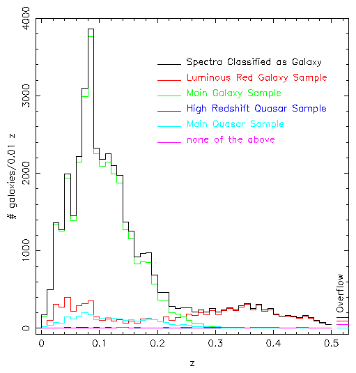
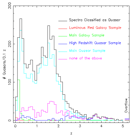
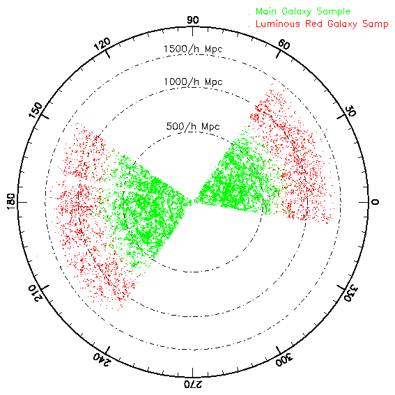
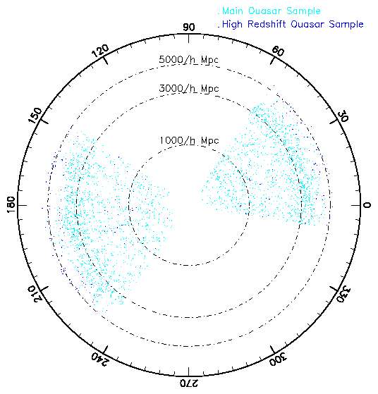
5 Beyond the Early Data Release
We encourage the active use of these data from the SDSS EDR. We have worked to make the data products as accurate as possible, but realize that some calibration or cataloging errors may have crept into our work. Feedback to the help desk set up at the STScI will allow us to evaluate the usefulness and correctness of these catalogs. As appropriate, we will update the calibration and contents of this early data release and announce these changes on the users' group mailing list and the SDSS web site.
The next data release of SDSS data is scheduled for January of 2003. It is scheduled to include at least 1,500 square degrees of imaging data and corresponding spectra.
The Sloan Digital Sky Survey (SDSS) is a joint project of The University of Chicago, Fermilab, the Institute for Advanced Study, the Japan Participation Group, The Johns Hopkins University, the Max-Planck-Institute for Astronomy (MPIA), the Max-Planck-Institute for Astrophysics (MPA), New Mexico State University, Princeton University, the United States Naval Observatory, and the University of Washington. Apache Point Observatory, site of the SDSS telescopes, is operated by the Astrophysical Research Consortium (ARC).
Funding for the project has been provided by the Alfred P. Sloan Foundation, the SDSS member institutions, the National Aeronautics and Space Administration, the National Science Foundation, the U.S. Department of Energy, the Japanese Monbukagakusho, and the Max Planck Society. The SDSS Web site is http://www.sdss.org/.
References
- [12001Anderson et al.]
-
Anderson, S. et al. 2001, , 122, 503
- [21980Bahcall & Soneira]
-
Bahcall, J. N. & Soneira, R. M. 1980, , 44, 73
- [31995Becker, White, & Helfand]
-
Becker, R. H., White, R. L., & Helfand, D. J. 1995, , 450, 559
- [42001aBlanton et al.]
-
Blanton, M. R., Dalcanton, J., Eisenstein, D. et al. 2001a,
AJ, 121, 2358
- [52001bBlanton et al.]
-
Blanton, M.R., Lupton, R.H., Maley, F.M., Young, N., Zehavi, I.,
& Loveday, J. 2001b, AJ, submitted (astro-ph/0105535)
- [61986Brodie & Hanes]
-
Brodie, J. P. & Hanes, D. A. 1986, , 300, 258
- [72001Calabretta & Greisen]
-
Calabretta, M. & Greisen, E.W., 2001, in preparation
- [82001Castander et al.]
-
Castander, Francisco J. et al. 2001, , 121, 2331
- [92001Chen et al.]
-
Chen, B., et al. 2001, , 553, 184
- [101995aConnolly et al.]
-
Connolly, A. J., Szalay, A. S., Bershady, M. A., Kinney, A. L.,
& Calzetti, D. 1995a, , 110, 1071
- [111995Connolly et al.]
-
Connolly, A. J., Csabai, I., Szalay, A. S., Koo, D. C., Kron, R. G.,
& Munn, J. A. 1995b, , 110, 2655
- [121999Connolly & Szalay]
-
Connolly, A.J., & Szalay, A.S. 1999, AJ, 117, 2052
- [132001Croom et al.]
-
Croom, S.M., Smith, R.J., Boyle, B.J. et al. 2001, MNRAS, 322, L29
- [142001Delaney]
-
Delaney, K. 2000, Inside Microsoft SQL Server 2000 (Microsoft Press)
- [151989Diaz, Terlevich, & Terlevich]
-
Diaz, A. I., Terlevich, E., & Terlevich, R. 1989, , 239, 325
- [162001Eisenstein et al.]
-
Eisenstein, D., et al. 2001, AJ, in press (astro-ph/0108153)
- [171999Fan]
-
Fan, X. 1999, , 117, 2528
- [181999Fan et al.]
-
Fan, X., Strauss, M. A., Schneider, D. P., et al. 1999, , 118, 1
- [192001aFan et al.]
-
Fan, X., Strauss, M. A., Richards, G. T., et al. 2001a, , 121, 31
- [202001bFan et al.]
-
Fan, X., Narayanan, V., Lupton, R.H., et al. 2001b, ,
in press (astro-ph/0108063)
- [212000Finlator et al.]
-
Finlator, K., Ivezi\'c, Z., Fan, X., et al. 2000, , 120, 2615
- [222000Fischer et al.]
-
Fischer, P., McKay, T., Sheldon, E., et al. 2000, , 120, 1198
- [231996Fukugita et al.]
-
Fukugita, M., Ichikawa, T., Gunn, J. E., Doi, M., Shimasaku, K., &
Schneider, D.P. 1996, , 111, 1748
- [241998Gunn et al.]
-
Gunn, J. E., Carr, M., Rockosi, C. et al. 1998, , 116, 3040
- [252001Hogg et al.]
-
Hogg, D. W., Schlegel, D., Finkbeiner, D. P., & Gunn, J. E.
2001, AJ, in press (astro-ph/0106511)
- [262000Høg et al.]
-
Høg, E., Fabricius, C., Makarov, V. V., Urban, S., Corbin, T.,
Wycoff, G., Bastian, U. Schwekendiek, P., & Wicenec, A. 2000,
, 355, L27
- [272000Ivezi\'c et al.]
-
Ivezi\'c, Z., Goldston, J., Finlator, K., et al. 2000, , 120, 963
- [282001Ivezi\'c et al.]
-
Ivezi\'c, Z., et al. 2001, AJ, in press (astro-ph/0105511)
- [292001Katgert]
-
Katgert, P. 2001, private communication
- [302000Kunszt et al.]
-
Kunszt, P., Szalay, A.S., Csabai, I., & Thakar, A. 2000,
in Proc ADASS IX, eds. N. Manset, C.Veillet, D. Crabtree,
(ASP Conference Series), 216, 141
- [312000Leggett et al.]
-
Leggett, S. et al. 2000, ApJ, 536, L35
- [322001cLupton et al.]
-
Lupton, R., Gunn, J. E., Ivezi\'c, Z., Knapp, G. R., Kent, S.,
& Yasuda, N. 2001,
in ASP Conf. Ser. 238, Astronomical Data Analysis Software and
Systems X, ed. F. R. Harnden, Jr., F. A. Primini, and H. E. Payne (San
Francisco: Astr. Soc. Pac.), in press (astro-ph/0101420)
- [332001aLupton et al.]
-
Lupton, R., et al. 2001a, in preparation
- [342001bLupton et al.]
-
Lupton, R., et al. 2001b, in preparation
- [351999Lupton et al.]
-
Lupton, R. H., Gunn, J. E., & Szalay, A. S. 1999, , 118 1406
- [362001Menou et al.]
-
Menou, K., Vanden Berk, D.E., Ivezi\'c, Z. et al. 2001, AJ, in press
(astro-ph/0102410)
- [371998Monet]
-
Monet, D.G. 1998, BAAS, 19312003
- [381997Newberg & Yanny]
-
Newberg, H.J., & Yanny, B. 1997, , 113, 89
- [392001Objectivity Inc.]
-
Objectivity Database Reference Manual, Objectivity Inc., Menlo Park, CA
- [401994Petravick et al.]
-
Petravick, D., Berman, E., MacKinnon, B., et al. 1994, SPIE, 2198, 935
- [411976Petrosian]
-
Petrosian, V. 1976, , 209, L1
- [421998Pickles]
-
Pickles, A. 1998, PASP, 110, 863
- [431856Pogson]
-
Pogson, N. R. 1856, , 17, 12
- [441995Postman & Lauer]
-
Postman, M., & Lauer, T.R. 1995, ApJ, 440, 28
- [452001aRichards et al.]
-
Richards, G.T., Fan, X., Schneider, D.P. et al. 2001a, AJ,
121, 2308
- [462001bRichards et al.]
-
Richards, G.T., et al. 2001b, in preparation
- [471992Rybicki & Press]
-
Rybicki, G.B. & Press, W.H. 1992, ApJ, 398, 169
- [481998Schlegel, Finkbeiner, & Davis]
-
Schlegel, D., Finkbeiner, D., & Davis, M. 1998, ApJ, 500, 525
- [492001Schneider et al.]
-
Schneider, D.P. et al. 2001, AJ, submitted
- [502001Scranton et al.]
-
Scranton, R., et al. 2001, ApJ, submitted (astro-ph/0107416)
- [511996Shectman et al.]
-
Shectman, S.A., Landy, S.D., Oemler, A., Tucker, D.L., Lin,
H., Kirshner, R.P., & Schechter, P.L. 1996, ApJ, 470, 172
- [522001Sheldon et al.]
-
Sheldon, E. et al. 2001, ApJ, 554, 881
- [532001Shimasaku et al.]
-
Shimasaku, K. et al. 2001, AJ, in press (astro-ph/0105401)
- [542001Smith et al.]
-
Smith, J. A., Tucker, D. L., Kent, S., et al. 2001, in preparation
- [551997Stark et al.]
-
Stark, J., Siebenmorgen, R., & Gredel, R. 1997, , 482, 1011
- [562001Strateva et al.]
-
Strateva, I. et al. 2001, AJ, in press (astro-ph/0107201)
- [572001Strauss et al.]
-
Strauss, M.A. et al. 2001, in preparation
- [582001Szalay et al.]
-
Szalay, A.S., Gray, J., Kunszt, P., Thakar, A., and Slutz, D. 2001, in Proceedings of MPA/MPE/ESO
Conference ``Mining the Sky'', Garching,
Germany
- [591979Tonry & Davis]
-
Tonry, J., & Davis, M. 1979, , 84, 1511
- [602000Thakar et al.]
-
Thakar,A., Kunszt, P.Z., Szalay, A.S. and Szokoly, G.P. 2001,
Multi-threaded Query Agent and Engine for a Very Large
Astronomical Database, in Proc ADASS IX, eds. N. Manset,
C. Veillet, D. Crabtree, ASP Conference series, 216,
231
- [611998Trager et al.]
-
Trager, S. C., Worthey, G., Faber, S. M., Burstein, D., & Gonzalez, J. J. 1998,
, 116, 1
- [622001Tucker et al.]
-
Tucker, D. L. et al. 2001, in preparation
- [632001Vanden Berk et al.]
-
Vanden Berk, D., et al. 2001, AJ, 122, 549
- [641999Voges et al.]
-
Voges, W., Aschenbach, B., Boller, Th., et al. 1999, , 349, 389
- [651998Waddell et al.]
-
Waddell, P. Mannery, E. J., Gunn, J. E., & Kent, S. M. 1998,
SPIE, 3352, 742
- [662000Yanny et al.]
-
Yanny, B., Newberg, H. J., Kent, S., et al. 2000, , 540, 825
- [672001Yasuda et al.]
-
Yasuda, N., Fukugita, M., Narayanan, V. et al. 2001, AJ, 122, 1104
- [682000York et al.]
-
York, D. G., Adelman, J., Anderson, J. E., et al. 2000, , 120, 1579
- [692001York et al.]
-
York, D. G. et al. 2001, in preparation
- [702000Zacharias et al.]
-
Zacharias, N., Urban, S. E., Zacharias, M. I., et al. 2000, , 120, 2131
- [712001Zehavi et al.]
- Zehavi, I., Blanton, M.R., Frieman, J.A. et al. 2001, , submitted (astro-ph/0106476)
| Latitude and Longitude | 32\arcdeg 46\arcmin 49.3\arcsecN, 105\arcdeg 49\arcmin 13.5\arcsecW |
| Elevation | 2788 meters |
| Survey Telescope | 2.5 meter diameter, modified Ritchey-Chrétien design; 27% central obscuration |
| Survey Area | NGP, 10,000 square degrees, minimal Galactic extinction |
| Plus three stripes in SGP | |
| Instruments | Imaging Camera and Two Double Spectrographs |
| Photometric Telescope | 20-inch, with 1 CCD camera, filter wheel, and shutter |
| Photometric CCDs | 30 2048 ×2048, SITe/Tektronix, 49.2 mm square |
| CCD Read Noise | < 5 electrons per pixel (overall system is sky limited) |
| Image frame size (pixels) | 2048×1361 pixels |
| Image frame size (arcmin) | 13.52 ×8.98 arcminutes |
| Image column separation | 25.17 arcminutes |
| Detector separation along column | 17.98 arcminutes |
| Focal plane image scale | 3.616 mm/arcmin |
| Detector image scale | 3.636 mm/arcmin |
| Pixel Size and scale | 24 micron; 0.396 arcsec/pixel |
| Filters | r i u z g scanned in that order, 71.7 seconds apart |
| Integration Time | 54 seconds |
| Operating Mode | Time Delay and Integrate (``Drift Scan'') |
| Field Distortion | < 0.1 arcsec over whole field |
| Field Size | 2.5 |
| Flux Calibration | Standard star fields at 15 intervals along scans, |
| tied to BD+17 4708, atmospheric extinction determined by PT. | |
| Astrometric CCDs | 22, 0.25 × 2 inch, above and below CCD columns, |
| r filter +3 mag ND filter, 10.5 sec. integration time | |
| Channels | One red, one blue for each spectrograph |
| CCDs | SITe/Tektronix (as for imager) |
| Coverage | 3800Å-6150Å (blue), 5800Å-9200Å (red), l/Dlapprox. 1800 |
| No. of fibers | 320×2 |
| Fiber diameter | 3 arcsec |
| Flux Calibration | Standard stars in each field, tied to colors observed with camera |
| Integration time | 45 minutes, in three exposures (nominal (S/N)2 per pixel > 15 at g*=20.2) |
| Pixel size | 69 km s-1 |
| Wavelength Calibration | Hg, Cd & Ne arclamps, RMS error of 0.07 pixel (10 km s-1) |
| Flat field | quartz lamps |
| PSF-FWHM | 1.2-2.3 arcsec |
| 95% completeness limit for point source | u*:22.0; g*:22.2; r*:22.2; i*:21.3; z*:20.5 |
| Sky Coverage within Survey Area | 98% (omitting areas around bright stars) |
| Photometric Calibration Errors for Point Sources | u*:5%; g*:3%; r*:3%; i*:3%; z*:5% |
| Star-Galaxy Separation | 95% correct at 21 magnitude in r* |
| Astrometric errors | Absolute: < 100 mas; Relative < 50 mas |
| (both rms per coordinate) | |
| Limiting magnitude | S/N=4.5/pixel at lfl=10-13 ergs/cm2/sec |
| Error in galaxy redshifts | Dz=0.0001 (approx. 30 km s-1) |
| Error in quasar redshifts | Dz=0.001 |
| Success rate, redshifts for galaxies | > 99% |
| Success rate, redshifts for quasars | 98% |
Table 3: Early Data Release Imaging Data
| Tile ID | Plate ID | Date Completed | RA (°) | DEC (°) | (S/N)2 at g*=20.2 | Smear Exposure |
| (MJD) | per pixel | Included? | ||||
| 122 | 266 | 51630 | 145.8928 | 0.0613 | 33.8 | No |
| 121 | 267 | 51608 | 147.7332 | -0.0307 | 31.1 | No |
| 120 | 268 | 51633 | 149.0618 | 0.0797 | 33.1 | No |
| 119 | 269 | 51910 | 150.6295 | 0.0000 | 22.8 | Yes |
| 118 | 270 | 51909 | 152.4607 | 0.0061 | 29.4 | No |
| 117 | 271 | - | 154.2643 | 0.0245 | - | - |
| 116 | 272 | 51941 | 156.0189 | 0.0184 | 24.8 | No |
| 115 | 273 | 51957 | 157.9021 | 0.0092 | 17.9 | No |
| 114 | 274 | 51913 | 159.7487 | 0.0184 | 65.7 | Yes |
| 113 | 275 | 51910 | 161.4664 | -0.0061 | 37.3 | Yes |
| 112 | 276 | 51909 | 163.3804 | 0.0429 | 47.1 | Yes |
| 111 | 277 | 51908 | 165.2300 | 0.0061 | 28.3 | Yes |
| 110 | 278 | 51900 | 167.0275 | 0.0276 | 47.1 | Yes |
| 109 | 279 | - | 168.8618 | -0.0061 | - | - |
| 108 | 280 | - | 170.4477 | 0.1655 | - | - |
| 107 | 281 | 51614 | 171.8773 | 0.1104 | 40.8 | No |
| 106 | 282 | 51658 | 173.7698 | -0.1196 | 33.8 | No |
| 105 | 283 | 51959 | 175.9750 | -0.0031 | 28.6 | No |
| 104 | 284 | 51943 | 177.9810 | -0.0644 | 27.8 | No |
| 103 | 285 | 51930 | 179.5608 | -0.0153 | 44.0 | Yes |
| 102 | 286 | 51999 | 181.3061 | 0.0092 | 16.5 | No |
| 101 | 287 | 52023 | 183.1557 | 0.0184 | 24.9 | No |
| 100 | 288 | 52000 | 184.8459 | -0.0184 | 20.5 | No |
| 99 | 289 | 51990 | 186.7078 | -0.0184 | 22.7 | No |
| 98 | 290 | 51941 | 188.9313 | 0.0307 | 20.4 | No |
| 97 | 291 | 51928 | 190.7257 | -0.0368 | 31.8 | Yes |
| 96 | 292 | 51609 | 192.5814 | -0.0245 | 21.4 | No |
| 95 | 293 | 51689 | 194.4555 | 0.0031 | 22.1 | No |
| 94 | 294 | 51986 | 196.5075 | 0.0889 | 22.8 | No |
| 93 | 295 | 51985 | 198.0996 | -0.0184 | 17.3 | No |
| 92 | 296 | 51665 | 199.8694 | 0.0674 | 17.3 | No |
| 91 | 297 | 51959 | 201.5658 | -0.0061 | 22.0 | Yes |
| 90 | 298 | - | 203.4644 | -0.0061 | - | - |
| 89 | 299 | 51671 | 205.3569 | 0.0061 | 31.9 | No |
| 88 | 300 | 51666 | 207.2249 | -0.0123 | 23.4 | No |
| 87 | 301 | 51942 | 209.6201 | -0.0552 | 30.9 | Yes |
| 86 | 302 | 51688 | 211.7208 | -0.0490 | 22.9 | No |
| 85 | 303 | 51615 | 213.4171 | 0.0674 | 24.2 | No |
| 84 | 304 | 51609 | 214.5129 | 0.0000 | 17.8 | Yes |
| 83 | 305 | 51613 | 216.3073 | 0.0337 | 24.2 | No |
| 82 | 306 | 51637 | 217.8810 | -0.0828 | 30.1 | No |
| 81 | 307 | 51663 | 219.7244 | 0.0552 | 24.9 | No |
| 80 | 308 | 51662 | 221.6415 | -0.0613 | 28.2 | No |
| 79 | 309 | 51994 | 223.6321 | 0.0245 | 32.0 | No |
| 78 | 310 | 51990 | 225.8618 | 0.0061 | 18.1 | No |
| 77 | 311 | 51665 | 227.2822 | 0.0245 | 22.5 | No |
| 76 | 312 | 51689 | 229.0766 | 0.0245 | 20.5 | No |
| 75 | 313 | 51673 | 230.9047 | -0.0215 | 22.7 | No |
| 74 | 314 | 51641 | 232.7451 | 0.0123 | 16.3 | No |
| 73 | 315 | 51663 | 234.5733 | -0.0031 | 18.6 | No |
| 97 | 324 | 51666 | 190.7257 | -0.0368 | 20.6 | No |
| 148 | 349 | 51699 | 254.1442 | 63.6530 | 47.4 | No |
| 149 | 350 | 51691 | 258.4975 | 65.1336 | 21.8 | No |
| 150 | 351 | 51780 | 255.9522 | 61.6193 | 22.0 | No |
| 151 | 352 | 51694 | 260.0012 | 63.0373 | 19.9 | No |
| 152 | 353 | 51703 | 257.5362 | 59.5647 | 37.1 | No |
| 153 | 354 | 51792 | 261.3024 | 60.9272 | 15.4 | Yes |
| 154 | 355 | 51788 | 258.9371 | 57.4932 | 28.9 | No |
| 155 | 356 | - | 262.4414 | 58.8061 | - | - |
| 156 | 357 | - | 260.1872 | 55.4078 | - | - |
| 157 | 358 | 51818 | 263.4490 | 56.6762 | 26.5 | Yes |
| 158 | 359 | 51821 | 261.3115 | 53.3110 | 18.9 | Yes |
| 159 | 360 | 51816 | 264.3484 | 54.5390 | 21.6 | Yes |
| 159 | 362 | 51999 | 264.3484 | 54.5390 | 27.9 | No |
| 74 | 363 | 51989 | 232.7451 | 0.0123 | 30.1 | No |
| 155 | 366 | 52017 | 262.4414 | 58.8061 | 18.4 | No |
| 156 | 367 | 51997 | 260.1872 | 55.4078 | 51.2 | No |
| 171 | 382 | - | 349.2559 | 0.0289 | - | - |
| 172 | 383 | 51818 | 351.2021 | 0.1141 | 28.3 | Yes |
| 173 | 384 | 51821 | 353.2949 | -0.0398 | 25.6 | Yes |
| 174 | 385 | 51877 | 355.3896 | 0.0444 | 52.4 | No |
| 175 | 386 | 51788 | 357.6322 | 0.0540 | 16.6 | No |
| 176 | 387 | 51791 | 359.8243 | 0.0243 | 35.3 | Yes |
| 177 | 388 | 51793 | 1.8246 | -0.0050 | 18.4 | Yes |
| 178 | 389 | 51795 | 3.5598 | -0.0248 | 26.3 | No |
| 179 | 390 | 51900 | 5.2229 | -0.0332 | 53.3 | Yes |
| 180 | 391 | 51782 | 6.9964 | 0.0453 | 18.7 | No |
| 181 | 392 | 51793 | 8.8956 | -0.0021 | 26.9 | Yes |
| 182 | 393 | 51794 | 10.8188 | 0.0369 | 23.6 | Yes |
| 183 | 394 | 51876 | 12.7276 | -0.0330 | 38.7 | Yes |
| 184 | 395 | 51783 | 14.6091 | 0.0160 | 22.3 | No |
| 185 | 396 | 51816 | 16.4703 | -0.0038 | 30.0 | Yes |
| 186 | 397 | 51794 | 18.2698 | 0.0185 | 29.0 | Yes |
| 187 | 398 | 51789 | 19.8354 | 0.0022 | 26.4 | Yes |
| 188 | 399 | 51817 | 21.6700 | 0.0376 | 28.3 | Yes |
| 189 | 400 | 51820 | 23.6367 | 0.0915 | 24.9 | Yes |
| 190 | 401 | 51788 | 25.8247 | -0.0208 | 23.2 | No |
| 191 | 402 | 51793 | 27.9064 | 0.0018 | 28.6 | Yes |
| 192 | 403 | 51871 | 29.8199 | 0.0102 | 24.8 | Yes |
| 193 | 404 | 51812 | 31.6460 | -0.0352 | 24.8 | Yes |
| 194 | 405 | 51816 | 33.6829 | -0.0329 | 20.2 | Yes |
| 195 | 406 | 51817 | 35.8830 | 0.1250 | 30.4 | Yes |
| 196 | 407 | 51820 | 37.8460 | -0.0594 | 30.4 | Yes |
| 197 | 408 | 51821 | 39.8224 | 0.0369 | 26.4 | Yes |
| 198 | 409 | 51871 | 41.9984 | 0.0040 | 33.5 | Yes |
| 199 | 410 | 51816 | 43.8616 | -0.0170 | 24.0 | Yes |
| 200 | 411 | 51817 | 45.7871 | -0.0168 | 26.3 | Yes |
| 201 | 412 | 51931 | 47.7341 | 0.0035 | 35.7 | Yes |
| 202 | 413 | 51929 | 49.6868 | 0.0153 | 33.2 | Yes |
| 203 | 414 | 51869 | 51.6314 | -0.0118 | 39.7 | Yes |
| 204 | 415 | 51810 | 53.5228 | 0.0307 | 25.7 | No |
| 205 | 416 | 51811 | 55.4916 | 0.0138 | 38.6 | Yes |
|
Class | Description | Table |
| PhotoObj | Imaging parameters | |
| PhotoPrimary | Primary Detections | |
| PhotoSecondary | Secondary Detections | |
| PhotoFamily | Bright or Blended Detections | |
| Tag | Tag Imaging parameters | |
| Primary | Primary Detections | |
| Star | Primary Star Detections | |
| Galaxy | Primary Galaxy Detections | |
| Sky | Primary Sky Objects | |
| Unknown | Primary, unknown identification | |
| Secondary | Secondary Detections | |
| StarSecondary | Secondary Star Detections | |
| GalaxySecondary | Secondary Galaxy Detections | |
| SkySecondary | Secondary Sky Objects | |
| UnknownSecondary | Secondary, unknown identification | |
| Family | Bright or Blended Detections | |
| ExternalCatalog | Objects matched from other catalogs | |
| ROSAT | ROSAT sources | |
| FIRST | FIRST radio sources | |
| USNO | USNO-A sources | |
| SpecObj | Spectroscopic parameters | |
| SpecLine | Spectroscopic lines | |
| SpecLineIndex | Index for spectroscopic lines | |
| CrossCorrelationRedshift | Measured cross-correlation redshifts | |
| EmissionRedshift | Measured emission line redshifts | |
| Statistics | Number of entries in the database | |
| Run | Statistics from one imaging run | |
| Chunk | Statistics from interleaved pair of runs | |
| Segment | One of twelve camera columns within a chunk | |
| Field | Summary of measured parameters for one imaging field | |
| Plate | Summary of parameters for one spectroscopic plate | |
| SDSSConstants | Definition of the survey geometry | |
|
|
Table 5: Summary of Database Classes
|
Name | Type | Description | In Tag? | |
|
| ||||
| Class PhotoObj: | ||||
| [4pt]
objID;id_;object_ID;obj_ID | int64 | The unique identifier for SDSS photometric objects. | Y | |
| A bit-encoded integer of run,rerun,camcol,field,objid. | ||||
| object;id;objid | int32 | The object id within a field (1-indexed) | N | |
| Usually changes between reruns of the same field. | ||||
| nChild;nchild;nChildren | int32 | Number of children if a deblended object. | Y | |
| BRIGHT objects also have nchild = 1, the non-BRIGHT sibling. | ||||
| objType;objc_type;objtype | int32 | Classification of the object. | Y | |
| ||||
| ||||
| ||||
| ||||
| ||||
| ||||
| ||||
| ||||
| ||||
| catID;catid;cat_ID | int32 | Catalog ID. Not used. | N | |
| objFlags;objc_flags;flag1; | int64 | Detection flags. See Table | Y | |
| objFlags2;objc_flags2;flag2 | See Table | |||
| rowC;objc_rowc;objRowc | float32 | Row center position - r coordinates. (pixels) | Y | |
| rowCErr;objc_rowcErr; | float32 | Row center position error - r coordinates. (pixels) | N | |
| objRowcErr | ||||
| colC;objc_colc;objColc | float32 | Column center position - r coordinates. (pixels) | Y | |
| colCErr;objc_colcErr; | float32 | Column center position error - r coordinates. (pixels) | N | |
| objColcErr | ||||
| rowV;rowv | float32 | Row-component of object's velocity. (deg/day) | N | |
| rowVErr;rowvErr | float32 | Error in row-component of object's velocity. (deg/day) | N | |
| colV;colv | float32 | Column-component of object's velocity. (deg/day) | N | |
| colVErr;colvErr | float32 | Error in column-component of object's velocity. (deg/day) | N | |
| row;rowc | float32[5] | Row center. (pixels) | N | |
| rowErr;rowcErr | float32[5] | Row center error. (pixels) | N | |
| col;colc | float32[5] | Column center. (pixels) | N | |
| colErr;colcErr | float32[5] | Column center error. (pixels) | N | |
| sky | float32[5] | Sky flux at center of object. (asinh mags/arcsec2) | N | |
| skyErr | float32[5] | Sky flux error. (asinh mags/arcsec2) | N | |
| psfMag;psfCounts | float32[5] | PSF flux. (asinh mags) | Y | |
| psfMagErr;psfCountsErr | float32[5] | PSF flux error. (asinh mags) | N | |
| fiberMag;fiberCounts | float32[5] | Flux in 3 arcsec diameter fiber radius. (asinh mags) | Y | |
| fiberMagErr;fiberCountsErr | float32[5] | Error in 3-arcsec fiber flux. (asinh mags) | N | |
| petroMag;petroCounts | float32[5] | Petrosian flux. (asinh mags) | Y | |
| petroMagErr;petroCountsErr | float32[5] | Petrosian flux error. (asinh mags) | N | |
| petroRad | float32[5] | Petrosian radius. (arcsec) | Y | |
| petroRadErr | float32[5] | Petrosian radius error. (arcsec) | N | |
| petroR50 | float32[5] | Radius containing 50% of Petrosian flux. (arcsec) | Y | |
| Note: Only petroR50[2] is in Tag Classes | ||||
| petroR50Err | float32[5] | (placeholder) | N | |
| petroR90 | float32[5] | Radius containing 90% of Petrosian flux. (arcsec) | Y | |
| Note: Only petroR90[2] is in Tag Classes | ||||
| petroR90Err | float32[5] | (placeholder) | N | |
| q;Q | float32[5] | Stokes Q parameter. | N | |
| qErr;QErr;Q_err | float32[5] | Stokes Q parameter error. | N | |
| u;U | float32[5] | Stokes U parameter. | N | |
| uErr;UErr;U_err | float32[5] | Stokes U parameter error. | N | |
| isoRowC;iso_rowc;isoRowc | float32[5] | Isophotal row centroid. (pixels) | N | |
| isoRowCErr;iso_rowcErr; | float32[5] | Isophotal row centroid error. (pixels) (placeholder) | N | |
| isoRowcErr | ||||
| isoRowCGrad;iso_rowcGrad; | float32[5] | Gradient in row centroid with isophote. | N | |
| isoRowcGrad | (pixels/(1 mag/arcsec2 SB change) at object center) | |||
| isoColC;iso_colc;isoColc | float32[5] | Isophotal column centroid. (pixels) | N | |
| isoColCErr;iso_colcErr; | float32[5] | Isophotal column centroid error. (pixels) (placeholder) | N | |
| isoColcErr | ||||
| isoColCGrad;iso_colcGrad; | float32[5] | Gradient in column centroid with isophote. | N | |
| isoColcGrad | (pixels/(1 mag/arcsec2 SB change) at object center) | |||
| isoA;iso_a | float32[5] | Isophotal major axis. (arcsec) | N | |
| isoAErr;iso_aErr | float32[5] | Isophotal major axis error. (arcsec) (placeholder) | N | |
| isoB;iso_b | float32[5] | Isophotal minor axis. (arcsec) | N | |
| isoBErr;iso_bErr | float32[5] | Isophotal minor axis error. (arcsec) (placeholder) | N | |
| isoAGrad;iso_aGrad | float32[5] | Gradient in major axis with isophote. | N | |
| (arcsec/(1 mag/arcsec2 SB change) at isophote) | ||||
| isoBGrad;iso_bGrad | float32[5] | Gradient in minor axis with isophote. | N | |
| (arcsec/(1 mag/arcsec2 SB change) at isophote) | ||||
| isoPhi;iso_phi | float32[5] | Isophotal position angle. (degrees (+N thru E)) | N | |
| isoPhiErr;iso_phiErr | float32[5] | Isophotal position angle error. (degrees) (placeholder) | N | |
| isoPhiGrad;iso_phiGrad | float32[5] | Gradient in positional angle with isophote. | N | |
| (degrees/(1 mag/arcsec2 SB change) at isophote) | ||||
| deVRad;r_deV | float32[5] | deVaucouleurs fit scale radius. (arcsec) | N | |
| deVRadErr;r_deVErr | float32[5] | deVaucouleurs fit scale radius error. (arcsec) | N | |
| deVaB;ab_deV | float32[5] | deVaucouleurs fit a/b. | N | |
| deVaBErr;ab_deVErr | float32[5] | deVaucouleurs fit a/b error. | N | |
| deVPhi;phi_deV | float32[5] | deVaucouleurs fit position angle. (degrees (+N thru E)) | N | |
| deVPhiErr;phi_deVErr | float32[5] | deVaucouleurs fit position angle error. (degrees) | N | |
| deVMag;counts_deV;deVCounts | float32[5] | deVaucouleurs mag fit. (asinh mags) | N | |
| deVMagErr;counts_deVErr; | float32[5] | deVaucouleurs mag fit error. (asinh mags) | N | |
| deVCountsErr | ||||
| expRad;r_exp | float32[5] | Exponential fit scale radius. (arcsec) | N | |
| expRadErr;r_expErr | float32[5] | Exponential fit scale radius error. (arcsec) | N | |
| expAB;ab_exp | float32[5] | Exponential fit a/b. | N | |
| expABErr;ab_expErr | float32[5] | Exponential fit a/b error. | N | |
| expPhi;exp_phi | float32[5] | Exponential fit position angle. (degrees (+N thru E)) | N | |
| expPhiErr;exp_phiErr | float32[5] | Exponential fit position angle error. (degrees) | N | |
| expMag;counts_exp;expCounts | float32[5] | Exponential fit. (asinh mags) | N | |
| expMagErr;counts_expErr; | float32[5] | Exponential fit error. (asinh mags) | N | |
| expCountsErr | ||||
| modelMag;counts_model;modelCounts | float32[5] | Better of DeV/Exp mag fit. (asinh mags) | N | |
| modelMagErr;counts_modelErr; | float32[5] | Better of DeV/Exp mag fit error. (asinh mags) | N | |
| modelCountsErr | ||||
| texture | float32[5] | Texture parameter (placeholder). | N | |
| lStar;star_L | float32[5] | Star log likelihood | Y | |
| Note: lStar_r;star_L_r in Tag Classes | ||||
| lExp;exp_L | float32[5] | Exponential disk fit log likelihood. | Y | |
| Note: lExp_r;exp_L_r in Tag Classes | ||||
| lDeV;deV_L | float32[5] | deVaucouleurs fit log likelihood. | Y | |
| Note: lDeV_r;deV_L_r in Tag Classes | ||||
| fracPSF | float32[5] | Fraction of light in PSF (placeholder). | N | |
| flags;flags2 | int64[5] | Same as objFlags, but for each band. | N | |
| type | int32[5] | Same as objType, but for each band. | N | |
| status | int32 | Bit mask specifying the status of the object. | Y | |
| AR_OBJECT_STATUS_SET | ||||
| Status has been set in reference to its own run. | ||||
| AR_OBJECT_STATUS_GOOD | ||||
| Good as determined by its object flags. | ||||
| Absence implies bad. | ||||
| AR_OBJECT_STATUS_DUPLICATE | ||||
| This object has one or more duplicate detections in | ||||
| an adjacent field of the same Frames Pipeline Run. | ||||
| AR_OBJECT_STATUS_OK_RUN | ||||
| Located in the primary range of rows for this field. | ||||
| AR_OBJECT_STATUS_RESOLVED | ||||
| This object has been resolved against other runs. | ||||
| AR_OBJECT_STATUS_PSEGMENT | ||||
| Belongs to a PRIMARY segment. | ||||
| Not neccessarily a primary object. | ||||
| AR_OBJECT_STATUS_FIRST_FIELD | ||||
| Belongs to the first field in its segment. | ||||
| AR_OBJECT_STATUS_OK_SCANLINE | ||||
| Lies within valid nu range for its scanline. | ||||
| AR_OBJECT_STATUS_OK_STRIPE | ||||
| Lies within valid eta range for its stripe. | ||||
| AR_OBJECT_STATUS_SECONDARY | ||||
| This is a secondary survey object. | ||||
| AR_OBJECT_STATUS_PRIMARY | ||||
| This is a primary survey object. | ||||
| AR_OBJECT_STATUS_TARGET | ||||
| This is a spectroscopic target. | ||||
| ra | float64 | J2000 right ascension (r). (degrees) | Y | |
| dec | float64 | J2000 declination (r). (degrees) | Y | |
| offsetRa | float32[5] | Filter-position RA minus final RA×cos(Dec). (arcsec) | N | |
| offsetDec | float32[5] | Filter-position Dec minus final Dec. (arcsec) | N | |
| primTarget | int32 | Bit mask specifying which primary target categories the | Y | |
| object was selected in. See Table for bit definitions. | ||||
| secTarget | int32 | Bit mask specifying which secondary target categories the | Y | |
| object was selected in. See Table for bit definitions. | ||||
| reddening | float32[5] | Reddening in each filter. (magnitudes) | Y | |
| priority | uint32 | Priority bits. | N | |
| rho | float32 | Surface brightness parameter (5 x log petro-rad_i). | Y | |
|
| ||||
| Database-specific outputs | ||||
| cx,cy,cz | float64 | Unit x,y,z-vector for RA+Dec. | Y | |
| htmID | int64 | Level 20 HTM ID | Y | |
| modelFluxID | int32 | KD-tree ID for flux space (model flux). | Y | |
| psfFluxID | int32 | KD-tree ID for flux space (PSF flux). | Y | |
| petroFluxID | int32 | KD-tree ID for flux space (Petrosian flux). | Y | |
| matchID | int64[] | List of the IDs of the matching objects. | N | |
| field;Field | OneAssoc(Field) | Link to the field that this object is in. | Y | |
| phototag;PhotoTag;tag | OneAssoc(PhotoTag) | Link to the tag object corresponding to this object. | N | |
| profile;Profile | OneAssoc(Profile) | Link to the profile parameters for this object. | Y | |
| externalcatalog;extern; | ManyAssoc | Link to external catalog associations, if any. | Y | |
| ExternalCatalog | (ExternalCatalog) | |||
| specobj;SpecObj;spec | ManyAssoc(SpecObj) | Link to spectroscopic object associations, if any. | Y | |
| child | ManyAssoc(PhotoObj) | Link to the deblended children of this object, if any. | Y | |
| parent | OneAssoc(PhotoObj) | Link to the parent object if this object has been deblended. | Y | |
| secondary | ManyAssoc(PhotoObj) | Link to all secondaries of this object if it is a primary. | Y | |
| primary | ManyAssoc(PhotoObj) | Link to the primary object(s) if this object is a secondary. | Y | |
| seclist | ManyAssoc(PhotoObj) | Link to other secondary objects if this is a secondary. | Y | |
| Note: The above Assoc(PhotoObj) type data members are Assoc(PhotoTag) in Tag Classes | ||||
| photoz;PhotoZ | OneAssoc(PhotoZ) | Link to the photometric redshift object (placeholder). | Y | |
| Note: The magnitudes below appear only in PhotoTag classes | ||||
| u | float64 | Better of DeV/Exp mag fit. (asinh mags) | Y | |
| g | float64 | Better of DeV/Exp mag fit. (asinh mags) | Y | |
| r | float64 | Better of DeV/Exp mag fit. (asinh mags) | Y | |
| i | float64 | Better of DeV/Exp mag fit. (asinh mags) | Y | |
| z | float64 | Better of DeV/Exp mag fit. (asinh mags) | Y | |
| Class Profile: | ||||
| The array of profile bins calculated for each photometric object | ||||
| nProf;nprof | int32[5] | Number of radial bins | ||
| u;profMean_u | float32[] | Mean flux in annulus, u band (maggies/arcsec2) | ||
| g;profMean_g | float32[] | Mean flux in annulus, g band (maggies/arcsec2) | ||
| r;profMean_r | float32[] | Mean flux in annulus, r band (maggies/arcsec2) | ||
| i;profMean_i | float32[] | Mean flux in annulus, i band (maggies/arcsec2) | ||
| z;profMean_z | float32[] | Mean flux in annulus, z band (maggies/arcsec2) | ||
| uErr;profErr_u | float32[] | Error of mean flux in annulus, u band (maggies/arcsec2) | ||
| gErr;profErr_g | float32[] | Error of mean flux in annulus, g band (maggies/arcsec2) | ||
| rErr;profErr_r | float32[] | Error of mean flux in annulus, r band (maggies/arcsec2) | ||
| iErr;profErr_i | float32[] | Error of mean flux in annulus, i band (maggies/arcsec2) | ||
| zErr;profErr_z | float32[] | Error of mean flux in annulus, z band (maggies/arcsec2) | ||
| photoobj;PhotoObj;obj;pobj | OneAssoc(sPhotoObj) | Link to the photometric object | ||
|
| ||||
|
aperture | radius | radius | area |
| (pixels) | (arcsec) | (pixels) | |
| 1 | 0.56 | 0.23 | 1 |
| 2 | 1.69 | 0.68 | 9 |
| 3 | 2.58 | 1.03 | 21 |
| 4 | 4.41 | 1.76 | 61 |
| 5 | 7.51 | 3.00 | 177 |
| 6 | 11.58 | 4.63 | 421 |
| 7 | 18.58 | 7.43 | 1085 |
| 8 | 28.55 | 11.42 | 2561 |
| 9 | 45.50 | 18.20 | 6505 |
| 10 | 70.15 | 28.20 | 15619 |
| 11 | 110.50 | 44.21 | 38381 |
| 12 | 172.50 | 69.00 | 93475 |
| 13 | 269.50 | 107.81 | 228207 |
| 14 | 420.50 | 168.20 | 555525 |
| 15 | 657.50 | 263.00 | 1358149 |
| Hex Bit | Flag | Explanation |
| 0x001 | INTERP | pixel's value has been interpolated |
| 0x002 | SATUR | pixel is/was saturated |
| 0x004 | NOTCHECKED | pixel was NOT examined for an object |
| 0x008 | OBJECT | pixel is part of some object |
| 0x010 | BRIGHTOBJECT | pixel is part of bright object |
| 0x020 | BINOBJECT | pixel is part of binned object |
| 0x040 | CATOBJECT | pixel is part of a catalogued object |
| 0x080 | SUBTRACTED | model has been subtracted from pixel |
| 0x100 | GHOST | pixel is part of a ghost |
| 0x200 | CR | pixel is part of a cosmic ray |
| Name | Hex Bit | Description |
| BRIGHT | 0x2 | Object was detected in first, ``bright'' object-finding |
| step; generally brighter than r* = 17.5 | ||
| SUBTRACTED | 0x100000 | This BRIGHT object had its wings subtracted from the frame |
| BINNED1 | 0x10000000 | This object was detected in the 1×1, unbinned image. |
| BINNED2 | 0x20000000 | This object was detected in the 2×2 binned image, |
| after unbinned detections are replaced by background. | ||
| BINNED4 | 0x40000000 | This object was detected in the 4×4 binned image. |
| EDGE | 0x4 | Object was too close to edge of frame |
| LOCAL_EDGE | 0x8000000000 | Center in at least one band is too close to an edge. |
| SATUR | 0x40000 | The object contains one or more saturated pixels |
| SATUR_CENTER | 0x80000000000 | The object center is close to at least one saturated pixel. |
| BLENDED | 0x8 | Object had multiple peaks detected within it; was |
| thus a candidate to be a deblending parent | ||
| NODEBLEND | 0x40 | No deblending was attempted on this object, even though it is BLENDED. |
| DEBLEND_TOO_MANY_PEAKS | 0x800 | There were more than 25 peaks in this object to |
| deblend; deblended brightest 25 | ||
| DEBLEND_PRUNED | 0x4000000 | At least one child was removed because its image was |
| too similar to a supposedly different child | ||
| PEAKS_TOO_CLOSE | 0x2000000000 | At least some peaks within this object were too close to be deblended, and |
| thus they were merged into a single peak. | ||
| DEBLEND_UNASSIGNED_FLUX | 0x40000000000 | After deblending, a significant fraction of flux was not assigned |
| to any children | ||
| DEBLENDED_AT_EDGE | 0x200000000000 | An object close enough to the edge of the frame that it normally |
| is not deblended is deblended anyway. Only set for objects large | ||
| enough to be EDGE in all fields/strips. | ||
| CHILD | 0x10 | Object is the product of an attempt to deblend a BLENDED object. |
| DEBLENDED_AS_PSF | 0x2000000 | The deblender treated this object as a PSF. |
| DEBLEND_NOPEAK | 0x400000000000 | There was no detected peak within this child in at least one band. |
| MOVED | 0x80000000 | The deblender identified this object as possibly moving. |
| DEBLENDED_AS_MOVING | 0x100000000 | A MOVED object that the deblender treated as moving |
| NODEBLEND_MOVING | 0x200000000 | A MOVED object that the deblender did not treat as moving |
| TOO_FEW_DETECTIONS | 0x400000000 | A child of this object was not detected in enough bands to reliably |
| deblend as moving | ||
| BAD_MOVING_FIT | 0x800000000 | The moving fit was too poor to be believable. |
| STATIONARY | 0x1000000000 | This object was consistent with being stationary. |
| BAD_MOVING_FIT_CHILD | 0x20000000000 | A possible moving child's velocity fit was too poor, so it was |
| discarded and the parent was not deblended as moving | ||
| TOO_FEW_GOOD_DETECTIONS | 0x1000000000000 | A child of this object had too few good detections to be deblended |
| as moving | ||
| PEAKCENTER | 0x20 | Given center is position of peak pixel, rather than |
| based on the maximum-likelihood estimator | ||
| CANONICAL_CENTER | 0x1 | Measurements used the center in r, rather than the locally determined center. |
| NOTCHECKED | 0x80000 | There are pixels in the object which were not checked |
| to see if they included a local peak, such as cores of saturated stars | ||
| MEDIAN_CENTRE | 0x4000000000 | Center given is of median-smoothed image |
| CENTER_OFF_AIMAGE | 0x2000000000000 | At least one peak's center lay off of the atlas image. This can |
| happen when the object is deblended as moving, or if the | ||
| astrometry is bad | ||
| NOPETRO | 0x100 | No valid Petrosian radius was found for this object. |
| MANYPETRO | 0x200 | More than one Petrosian radius was found. |
| NOPETRO_BIG | 0x400 | Petrosian radius is beyond the last point in the radial profile. |
| PETROFAINT | 0x800000 | At least one possible Petrosian radius was rejected as the |
| surface brightness at rP was too low. If NOPETRO isn't | ||
| set, a different, acceptable Petrosian radius was found. | ||
| MANYR50 | 0x2000 | An object has more than one 50% light radius |
| MANYR90 | 0x4000 | An object has more than one 90% light radius |
| BADSKY | 0x400000 | The sky level is so bad that the highest pixel in the object is |
| very negative; far more so than a mere non-detection. | ||
| No further analysis is attempted. | ||
| NOPROFILE | 0x80 | This object was too small or too close to the |
| edge to estimate a radial profile | ||
| TOO_LARGE | 0x1000000 | The object is too large for us to measure its profile (i.e. |
| it extends beyond a radius of approximately 260), | ||
| or at least one child is larger than half a frame | ||
| BAD_RADIAL | 0x8000 | Some of the points in the given radial profile have |
| negative signal-to-noise ratio. Not a significant parameter. | ||
| INCOMPLETE_PROFILE | 0x10000 | The Petrosian radius intersects the edge of the frame |
| ELLIPFAINT | 0x8000000 | The object's center is fainter than the isophote whose |
| shape is desired, so the isophote properties are not measured. | ||
| Also flagged if profile is incomplete. | ||
| CR | 0x1000 | Contains a pixel interpreted to be part of a cosmic ray. |
| INTERP | 0x20000 | The object contains one or more pixels whose values |
| were determined by interpolation | ||
| INTERP_CENTER | 0x100000000000 | The object center is close to at least one interpolated pixel. |
| PSF_FLUX_INTERP | 0x800000000000 | Greater than 20% of the PSF flux is from interpolated pixels. |
| BAD_COUNTS_ERROR | 0x10000000000 | An object containing interpolated pixels had too few good pixels |
| to form a reliable estimate of its error; the quoted error | ||
| may be underestimated | ||
| NOSTOKES | 0x200000 | No Stokes parameter was measured, either because of an |
| incomplete profile or numerical difficulties. | ||
|
|
Table 9: Processing flags associated with Measuring Objects in frames
|
| ||
| Class ExternalCatalog: | ||
| External Object | ||
| delta | float32 | Position difference between catalog and r photo object (arcsec) |
| match | int32 | Match to different catalogs |
| USNO : 1 = match to catalog within 30" | ||
| FIRST: number of matches to catalog within 1.5" | ||
| ROSAT: 1 = match to catalog within 60" | ||
| type | int16 | Object match type |
| ROSAT_MATCH = 0 | ||
| FIRST_MATCH = 1 | ||
| USNO_MATCH = 2 | ||
| phototag;PhotoTag;obj;pobj | OneAssoc(PhotoTag) | Link to photo tag object |
| Class FIRST: | ||
| SDSS objects that match to FIRST objects have their match parameters stored here. | ||
| Inherits everything from ExternalCatalog, plus has: | ||
| peak;firstPeak | float32 | Peak first radio flux (mJy) |
| integr;int;firstInt | float32 | Integrated first radio flux (mJy) |
| rms;firstRms | float32 | rms error in flux (mJy) |
| major;firstMajor | float32 | Major axis (deconvolved) (arcsec) |
| minor;firstMinor | float32 | Minor axis (deconvolved) (arcsec) |
| pa;firstPa | float32 | position angle (east of north) (degrees) |
| id;firstId | int32 | FIRST catalog id of one matching source |
| lambda | float64 | Composite radio source survey longitude (degrees) |
| eta | float64 | Composite radio source survey latitude (degrees) |
| Class ROSAT: | ||
| SDSS objects that match to Rosat objects have their match parameters stored here. | ||
| Inherits everything from ExternalCatalog, plus has: | ||
| cps;rosatCps | float32 | integrated ROSAT counts (counts/sec) |
| hard1;rosatHr1;hr1 | float32 | ROSAT hardness ratio 1 |
| hard2;rosatHr2;hr2 | float32 | ROSAT hardness ratio 2 |
| extent;rosatExt;ext | float32 | ROSAT extent parameter (arcsec) |
| exposure;rosatExposure | float32 | ROSAT exposure time (seconds) |
| posErr;rosatPosErr;poserr | float32 | Error in ROSAT position (arcsec) |
| cpsErr;rosatCpsErr;cpserr | float32 | Error in integrated ROSAT counts (counts/sec) |
| hard1Err;rosatHr1Err;hr1Err | float32 | Error in ROSAT hardness ratio 1 |
| hard2Err;rosatHr2Err;hr2Err | float32 | Error in ROSAT hardness ratio 2 |
| extentLike;rosatExtLike | float32 | ROSAT extent parameter likelihood |
| detectLike;rosatDetectLike | float32 | ROSAT detection likelihood |
| Class USNO: | ||
| SDSS objects that match to USNOA2.0 objects have their match parameters stored here. | ||
| Inherits everything from ExternalCatalog, plus has: | ||
| propermotion | float32 | Proper motion of object (arcsec/century) |
| angle;propermotionangle | float32 | Direction of proper motion (degrees (+N through E)) |
| blue;usnoBlue | float32 | Blue magnitude of matching USNO object (mag) |
| red;usnoRed | float32 | Red magnitude of matching USNO object (mag) |
|
| ||
|
| |||
| Class SpecObj: | |||
| Spectroscopic Object | |||
| specobj_ID;spec_ID | int64 | Unique ID | |
| xFocal | float64 | X Focal position on plate (mm) | |
| yFocal | float64 | Y Focal position on plate (mm) | |
| fiberID | int16 | Fiber ID (1-640) | |
| z | float32 | Final Redshift (heliocentric) | |
| zErr;z_err | float32 | Redshift error | |
| zConf;z_conf | float32 | Redshift confidence (between 0 and 1) | |
| zStatus;z_status | int16 | Redshift status: | |
| |||
| |||
| |||
| |||
| |||
| |||
| |||
| |||
| |||
| |||
| |||
| |||
| specClass;spec_cln | int16 | Spectral classification: | |
| |||
| |||
| |||
| |||
| |||
| |||
| |||
| |||
| zWarning;z_warnin | uint32 | Bit mask for warning flags: | |
| |||
| |||
| |||
| |||
| |||
| |||
| |||
| |||
| |||
| |||
| |||
| |||
| |||
| |||
| |||
| |||
| |||
| velDisp;vel_dis | float32 | Velocity dispersion (km/s) (placeholder) | |
| velDispErr;vel_dise | float32 | Velocity dispersion error (km/s) (placeholder) | |
| eCoeff;ecoeff | float32[5] | Expansion coefficients for galaxies | |
| eClass;eclass | float32 | Classification | |
| nGood | int32 | Number of good pixels in spectrum | |
| sn | float32[3] | Median S/N in g,r,i | |
| mag | float32[3] | Synthetic magnitude in g*,r*,i* | |
| ra | float64 | RA (degrees) | |
| dec | float64 | Dec (degrees) | |
| htmID | int64 | HTM ID | |
| fiberCounts | float32[5] | Fiber magnitudes (asinh magnitudes) | |
| objID | int64 | SDSS ID of object | |
| primTarget | int32 | Primary target flag (Table ) | |
| secTarget | int32 | Secondary target flag | |
| pixMin | int16 | Minimum pixel number | |
| pixMax | int16 | Maximum pixel number | |
| objType | char[32] | Object type as string | |
| phototag;PhotoTag;obj;tag | OneAssoc(PhotoTag) | Link to corresponding photometric object | |
| emissionredshift;elz;emz; | ManyAssoc | Link to the emission-line redshift measures | |
| EmissionRedshift | (EmissionRedshift) | ||
| crosscorrelationredshift; | ManyAssoc | Link to the redshifts from cross-correlations | |
| CrossCorrelationRedshift; | (CrossCorrelation- | ||
| xcorrz;xcz | Redshift) | ||
| found | ManyAssoc(SpecLine) | Link to found spectral lines | |
| measured | ManyAssoc(SpecLine) | Link to measured spectral lines | |
| speclineindex;lineidx; | ManyAssoc | Link to spectral line indices | |
| SpecLineIndex | (SpecLineIndex) | ||
| plate;Plate | OneAssoc(Plate) | Link to corresponding plate object | |
|
| |||
|
| ||
| Class SpecLine: (in observed frame) | ||
| Identified Spectroscopic Lines | ||
| specline_ID | int64 | Unique ID |
| wave | float32 | Line center (Å) |
| waveErr | float32 | Error in line center (Å) |
| waveMin | float32 | Minimum wavelength of line influence (Å) |
| waveMax | float32 | Maximum wavelength of line influence (Å) |
| sigma | float32 | Sigma of fitted gaussian (Å) |
| sigmaErr | float32 | Error of sigma (Å) |
| sigmaMin | float32 | Minimum sigma allowed by fit (Å) |
| sigmaMax | float32 | Maximum sigma allowed by fit (Å) |
| height | float32 | Height of gaussian (10-17 erg/s/cm2/Å) |
| heightErr | float32 | Error in height (10-17 erg/s/cm2/Å) |
| continuum | float32 | Continuum value at this pixel (10-17 erg/s/cm2/Å) |
| ew | float32 | Equivalent width (Å) |
| ewErr | float32 | Error in equivalent width (Å) |
| ewMin | float32 | Minimum equivalent width allowed for line detection (Å) |
| specIndex | float32 | Spectral index (not used) |
| nSigma | float32 | Significance of line number of sigma (not used) |
| chisq | float32 | c2 of fit |
| nu | int16 | Number of degrees of freedom |
| restWave | float32 | Line rest wavelength (Å) |
| weight | float32 | Weight of line in redshift determination |
| z | float32 | Redshift of line (heliocentric) |
| zErr | float32 | Error in redshift |
| lineMask | uint32 | Line mask (not used) |
| category | int16 | Category: Line found (0) or measured (1) |
| specobj;spec | OneAssoc(SpecObj) | Link to spectrum object |
| speclinename;linename;name | OneAssoc(SpecLineName) | Link to line name |
| Class SpecLineName: | ||
| Names of spectral lines | ||
| lineID | int32 | Line ID |
| restWave | float32 | Line rest wavelength (Å) |
| name | char[16] | Line name |
| Class SpecLineIndex: (in rest frame) | ||
| Spectral Indices | ||
| speclineindex_ID | int64 | Unique ID |
| name | char[16] | Name |
| ew | float32 | Equivalent width (Å) or flux ratio |
| ewErr | float32 | Equivalent width error (Å) |
| mag | float32 | Magnitude (2.5 log(EW)) of the line index |
| magErr | float32 | Magnitude error |
| waveMin | float32 | Minimum rest wavelength used to calculate the index |
| waveMax | float32 | Maximum rest wavelength used to calculate the index |
| z | float32 | Redshift |
| sn | float32 | Signal-to-noise ratio |
| specobj;spec | OneAssoc(SpecObj) | Link to spectrum object |
| Class CrossCorrelationRedshift: | ||
| Results of cross-correlation redshift measurement | ||
| crosscorrelationredshift_ID;xcz_ID | int64 | Unique ID |
| tempNo;temp_no | int16 | Template number |
| peakNo;peak_no | int16 | Peak number |
| shift | float32 | Number of pixels between object and template |
| z | float32 | Redshift from this peak |
| zErr;z_err | float32 | Error in redshift |
| r | float32 | Tonry & Davis r |
| zConf;con;conf;z_conf | float32 | Confidence |
| height | float32 | Height of CCF Peak |
| width | float32 | Width of CCF Peak |
| widthErr;width_err | float32 | Error in CCF width |
| delta | float32 | Error in CCF Peak |
| rms | float32 | RMS of CCF |
| specobj;spec | OneAssoc(SpecObj) | Link to spectrum object |
| Class EmissionRedshift: | ||
| Results of emission line redshift measurement | ||
| emissionredshift_ID;emz_ID | int64 | Unique ID |
| z | float32 | Redshift |
| zErr | float32 | Error in redshift |
| zConf | float32 | Confidence in redshift |
| nFit | int32 | Number of matched lines |
| wtFit;fitWeight | float32 | Weight of fit |
| specobj;spec | OneAssoc(SpecObj) | Link to spectrum object |
|
| ||
| Hex Bit | Flag | Explanation |
| Flags set on the entire spectrum | ||
| 0x001 | NOPLUG | Fiber not listed in plugmap file |
| 0x002 | BADTRACE | Bad trace of flatfield |
| 0x004 | BADFLAT | Low counts in fiberflat |
| 0x008 | BADARC | Bad arc solution |
| 0x010 | MANYBADCOLUMNS | > 10% of pixels are bad columns |
| 0x020 | MANYREJECTED | > 10% of pixels are rejected in extraction |
| 0x040 | LARGESHIFT | Large spatial shift between flat and object position |
| 0x080 | BADSKYFIBER | Sky Fiber shows extreme residuals |
| 0x100 | NEARWHOPPER | Within 2 fibers of a very bright object |
| 0x400 | SMEARIMAGE | Smear available for red and blue cameras |
| 0x800 | SMEARHIGHSN | S/N sufficient for full smear fit |
| 0x1000 | SMEARMEDSN | S/N only sufficient for scaled median fit |
| Flags set on single pixels | ||
| 0x10000 | NEARBADPIXEL | Bad pixel within 3 pixels of trace |
| 0x20000 | LOWFLAT | Flat field less than 0.5 |
| 0x40000 | FULLREJECT | Pixel fully rejected in extraction |
| 0x80000 | PARTIALREJECT | Some pixels rejected in extraction |
| 0x100000 | SCATTEREDLIGHT | Scattered light significant |
| 0x200000 | CROSSTALK | Cross-talk significant |
| 0x400000 | NOSKY | Sky level unknown at this wavelength |
| 0x800000 | BRIGHTSKY | Sky level > flux + 10*(flux error) |
| AND sky > 1.25*median sky over 99 pixels | ||
| 0x1000000 | NODATA | No data available in combine B-spline |
| 0x2000000 | COMBINEREJ | Rejected in combine B-spline |
| 0x4000000 | BADFLUXFACTOR | Low flux-calibration or flux-correction factor |
| 0x8000000 | BADSKYCHI | c2 > 4 in sky residuals at this wavelength |
| 0x10000000 | REDMONSTER | Contiguous region of bad c2 in sky residuals |
|
Name | Type | Description |
| Class Statistics: | ||
| Total number of chunks, runs, fields, objects and segments | ||
| nChunk | int32 | Number of chunk objects |
| nRun | int32 | Number of run objects |
| nSegment | int32 | Number of segments |
| nField | int32 | Number of fields |
| nPhotoObj | int32 | Number of Photo Objects |
| nPrimary | int32 | Number of Primary Photo Objects |
| nSecondary | int32 | Number of Secondary Photo Objects |
| nFamily | int32 | Number of Family Objects |
| nStar | int32 | Number of objects classified as stars |
| nGalaxy | int32 | Number of obects classified as galaxies |
| nSky | int32 | Number of objects classified as sky |
| nUnknown | int32 | Number of objects classified as unknown |
| nStarSec | int32 | Number of secondary objects classified as star |
| nGalaxySec | int32 | Number of secondary objects classified as galaxy |
| nSkySec | int32 | Number of secondary objects classified as sky |
| nUnknownSec | int32 | Number of secondary objects classified as unknown |
| nExternal | int32 | Number of external objects |
| nPlate | int32 | Number of plates |
| nSpecObj | int32 | Number of spectra |
| nSpecLine | int32 | Number of spectral lines |
| nSpecLineIndex | int32 | Number of spectral line indices |
|
| ||
| Name | Type | Description |
| Class Run: | ||
| One continuous photometric observation | ||
| run;runNumber | int32 | Run number |
| skyNodes | int64[] | Level 5 HTM nodes of this run |
| chunk;Chunk | ManyAssoc(sxChunk) | Link to the chunks this run is part of |
| segment;Segment | ManyAssoc(sxSegment) | Link to the segments of this run |
| Class Chunk: | ||
| Completely observed pair of strips | ||
| chunkNumber | int16 | Chunk number |
| startMu | int32 | Starting coordinate in Great Circle coordinates |
| endMu | int32 | Ending coordinate in Great Circle coordinates |
| stripe | int32 | Stripe number |
| exportVersion | char[32] | Export version |
| segment;Segment | ManyAssoc(sxSegment) | Link to all segments of this chunk |
| Class Segment: | ||
| A single camera column within a chunk | ||
| segment_ID;id;segID | int64 | Unique segment identifier |
| run | int32 | Run number of this segment |
| camCol | int32 | Camera column number (1-6) |
| rerun | int32 | Rerun number |
| field0 | int32 | Starting field number |
| nFields | int32 | Number of fields in segment |
| dscale | int32 | Scaling for bias |
| strip | int16 | Strip (N or S) |
| status | int16 | Status: primary,secondary or bad |
| resolved | int16 | Resolved flag (yes/no) |
| exported | int16 | Exported flag (yes/no) |
| families | int16 | Families identified flag (yes/no) |
| loadMJD | float64 | Date / Time at loading of database |
| equinox | float64 | Great Circle Equinox |
| node | float64 | Great Circle Ascending Node |
| incl | float64 | Great Circle Inclination |
| cObs;c_obs | float64 | CCD Clock rate |
| tracking | float64 | Tracking Rate |
| raMin;ramin | float64 | Lowest J2000 RA (degrees) |
| raMax;ramax | float64 | Highest J2000 RA (degrees) |
| decMin;decmin | float64 | Lowest J2000 Dec (degrees) |
| decMax;decmax | float64 | Highest J2000 Dec (degrees) |
| lMin;lmin | float64 | Lowest Galactic longitude (degrees) |
| lMax;lmax | float64 | Highest Galactic longitude (degrees) |
| bMin;bmin | float64 | Lowest Galactic latitude (degrees) |
| bMax;bmax | float64 | Highest Galactic latitude (degrees) |
| lambdaMin;lambdamin | float64 | Lowest survey l (degrees) |
| lambdaMax;lambdamax | float64 | Highest survey l (degrees) |
| etaMin;etamin | float64 | Lowest survey h (degrees) |
| etaMax;etamax | float64 | Highest survey h (degrees) |
| photoId;photo_id | char[32] | Photo ID tag |
| photoVersion;phot_ver | char[32] | Photo version |
| targetAstroId;tast_id | char[32] | Astrometric pipeline used for target |
| targetAstroVersion;tast_ver | char[32] | Astrometric pipeline version used for target selection |
| exportAstroId;eastr_id | char[32] | Astrometric calibration used for export to SX. |
| exportAstroVersion;eastr_ver | char[32] | Astrometric pipeline version used for export to SX. |
| targetFCalibId;tfcal_id | char[32] | Photometric calibration used for target selection. |
| targetFCalibVersion;tfcal_ver | char[32] | FCALIB pipeline version used for target selection |
| exportFCalibId;efcal_id | char[32] | Photometric calibration used for export to SX. |
| exportFCalibVersion;efcal_ver | char[32] | FCALIB pipeline version used for export to SX. |
| sxLoaderVersion; | char[32] | Version of SX Loader used to load this segment |
| loaderVersion;load_ver | ||
| objectSource;obj_src | char[32] | Object Source |
| targetSource;targ_src | char[32] | Target Source |
| targetVersion | char[32] | Target version |
| skyMask_;skyMask | uint32[] | BitMask encoded HTM nodes covered by this segment |
| skyMaskLength_;skyMaskLength | uint32 | Length of BitMask |
| field;Field | ManyAssoc(sxField) | Link to fields in this segment |
| chunk;Chunk | OneAssoc(sxChunk) | Link to the chunk this segment belongs to |
|
| ||
|
Name | Type | Description | |
| Class Field: | |||
| All the measured parameters of a photometric field | |||
| fieldID;id,;field_ID | int64 | Unique field identifier: Bitmask consisting of | |
| run,rerun,camcol,fieldnumber | |||
| field;fieldNumber | int32 | Field number | |
| nObjects;nobj | int32 | Number of objects in the field | |
| nDetectedObjects;ndetected | int32 | Number of objects actually detected | |
| nChild;nchild | int32 | Number of `child' objects | |
| nGalaxy;nGals;ngals;ngalaxy;n_gals | int32 | Number of objects classified as `galaxy' | |
| nStars;nstars;n_stars | int32 | Number of objects classified as `star' | |
| numStars;numstars;num_stars | int32[5] | Number of stars found in each band | |
| nCR;n_CR | int32[5] | Number of cosmic rays in each band | |
| nBrightObj;n_bright_obj | int32[5] | Number of bright objects in each band | |
| nFaintObj;n_faint_obj | int32[5] | Number of faint (nonbright) objects in each band | |
| quality | int32 | Data quality: | |
| |||
| |||
| |||
| |||
| |||
| mjd;MJD | float64[5] | MJD(TAI) when row 0 was read. | |
|
| |||
| Astrometric calibration quantities | |||
| a | float64[5] | Astrometric transformation constants. | |
| b | float64[5] | Astrometric transformation constants. | |
| c | float64[5] | Astrometric transformation constants. | |
| d | float64[5] | Astrometric transformation constants. | |
| e | float64[5] | Astrometric transformation constants. | |
| f | float64[5] | Astrometric transformation constants. | |
| dRow0;d_row0 | float64[5] | Zero-order row distortion coefficient. | |
| dRow1;d_row1 | float64[5] | First-order row distortion coefficient. | |
| dRow2;d_row2 | float64[5] | Second-order row distortion coefficient. | |
| dRow3;d_row3 | float64[5] | Third-order row distortion coefficient. | |
| dCol0;d_col0 | float64[5] | Zero-order column distortion coefficient. | |
| dCol1;d_col1 | float64[5] | First-order column distortion coefficient. | |
| dCol2;d_col2 | float64[5] | Second-order column distortion coefficient. | |
| dCol3;d_col3 | float64[5] | Third-order column distortion coefficient. | |
| csRow;cs_row | float64[5] | Slope in row DCR correction for blue objects. | |
| csCol;cs_col | float64[5] | Slope in column DCR correction for blue objects | |
| ccRow;cc_row | float64[5] | Constant row DCR correction for red objects. | |
| ccCol;cc_col | float64[5] | Constant column DCR correction for red objects. | |
| riCut;ri_cut | float64[5] | r*-i* cutoff between blue and red objects. | |
| airmass;air_mass;airMass | float64[5] | Airmass for star at frame center (mid exposure) | |
| raMin;ra_min | float64 | Minimum RA of field (degrees) | |
| raMax;ra_max | float64 | Maximum RA of field (degrees) | |
| decMin;dec_min | float64 | Minimum Dec of field (degrees) | |
| decMax;dec_max | float64 | Maximum Dec of field (degrees) | |
| scanlineArea;scanLineArea; | float32 | Area of scanline covered by the field (deg2) | |
| scanline_area | |||
| stripeArea;stripe_area | float32 | Area of stripe covered by the field (deg2) | |
|
| |||
| Photometric calibration quantities | |||
| seqID;seqId | int32 | Sequence id overlapping this field (-1=none) | |
| aa | float32[5] | Zero-point. | |
| aaErr;aa_err | float32[5] | Zero-point error | |
| bb | float32[5] | Color term. | |
| bbErr;bb_err | float32[5] | Color term error | |
| cc | float32[5] | Color x extinction term. | |
| ccErr;cc_err | float32[5] | Error in color extinction term. | |
| kk | float32[5] | Extinction coefficient. | |
| kkErr;kk_err | float32[5] | Error in extinction coefficient. | |
|
| |||
| framesStatus;frames_status | int32 | Info from the fpFieldStat file : Frames Processing Status | |
| rowOffset;row_offset | float32[5] | Offset to add to transformed row coordinates (pixels). | |
| colOffset;col_offset | float32[5] | Offset to add to transformed column coordinates (pixels). | |
| saturationLevel;saturation_level | int32[5] | Saturation level (counts) | |
| culled | int32 | Bit mask with the same values as primTarget, Table . | |
| A set bit indicates that targets of that type were culled | |||
| from the field, and therefore that field is excluded from that | |||
| particular science sample. | |||
| badMask, acceptableMask, | int32 | The four unsigned 32-bit integer bit masks ``badMask", | |
| goodMask, holeMask | ``acceptableMask", ``goodMask", and ``holeMask" indicate | ||
| which quality categories were of the specified quality | |||
| for each field. The bits are enumerated as follows: | |||
| |||
| |||
| |||
| |||
| |||
| |||
| |||
| |||
| |||
| |||
| |||
| |||
| |||
| |||
| |||
| |||
| |||
| |||
| |||
| |||
| |||
| |||
| gain | float32[5] | Gain averaged over amplifiers (electrons/DN) | |
| darkVariance;dark_variance | float32[5] | Dark variance | |
| acceptableMask | int32 | See description of badMask | |
| goodMask | int32 | See description of badMask | |
| holeMask | int32 | See description of badMask | |
|
| |||
| Outputs of PSP | |||
| skyPsp;sky_psp | float32[5] | Sky from the point spread function fit. (asinh mags/arcsec2) | |
| skyFrames;sky_frames | float32[5] | Global sky value in the corrected frame. (asinh mags/arcsec2) | |
| skyFramesSub;sky_frames_sub | float32[5] | Global sky value after object subtraction. (asinh mags/arcsec2) | |
| sky | float32[5] | Average sky in frame (asinh mags/arcsec2) | |
| skySig;sky_sig | float32[5] | Sigma of sky value distribution (asinh mags/arcsec2) | |
| skyErr;sky_err | float32[5] | Error of average sky in frame. (asinh mags/arcsec2) | |
| skySlope;sky_slope | float32[5] | Slope in sky value along columns (asinh mags/arcsec2/field) | |
| lbias;lBias;l_bias | float32[5] | Left-hand bias level (ADUs x DSCALE) | |
| rbias;rBias;r_bias | float32[5] | Right-hand bias level (ADUs x DSCALE) | |
| sigPix;sky_pix | float32[5] | Clipped s of pixel values in corrected frame (asinh mags/arcsec2) | |
| deVApCorrection;deV_ap_correction | float32[5] | deVaucouleurs aperture correction (mag) | |
| deVApCorrectionErr; | float32[5] | deVaucouleurs aperture correction error (mag) | |
| deV_ap_correctionErr | |||
| expApCorrection;exp_ap_correction | float32[5] | exponential aperture correction (mag) | |
| expApCorrectionErr; | float32[5] | exponential aperture correction error (mag) | |
| exp_ap_correctionErr | |||
| deVModelApCorrection; | float32[5] | deVaucouleurs model aperture correction (mag) | |
| deV_model_ap_correction | |||
| deVModelApCorrectionErr; | float32[5] | deVaucouleurs model aperture correction error (mag) | |
| deV_model_ap_correctionErr | |||
| expModelApCorrection; | float32[5] | Exponential model aperture correction (mag) | |
| exp_model_ap_correction | |||
| expModelApCorrectionErr; | float32[5] | Exponential model aperture correction error (mag) | |
| exp_model_ap_correctionErr | |||
| medianFiberColor;median_fiberColor; | float32[5] | Median fiber colors of objects in field (mag) | |
| median_fiber_color | |||
| medianPsfColor;median_psfColor; | float32[5] | Median PSF colors of objects in field (mag) | |
| median_psf_color;medianPSFColor | |||
| q;Q | float32[5] | Mean Stokes Q parameter on the frame | |
| u;U | float32[5] | Mean Stokes U parameter on the frame | |
|
| |||
| PSF fitting details | |||
| status | int32[5] | Type of PSF fit for each filter in the field | |
| |||
| |||
| |||
| |||
| |||
| |||
| |||
| pspStatus;psp_status | int16 | Maximum value of ``status'' over all 5 filters. | |
| psfNStar;psf_nstar | int32[5] | Number of stars used in PSF measurement. | |
| nEffPsf;nEffPSF;neff_psf | float32[5] | Effective area of the point spread function. (pixels) | |
| psfApCorrectionErr; | float32[5] | Photometric error due to imperfect PSF model (mags) | |
| psf_ap_correctionErr | |||
| psfSigma1;psf_sigma1 | float32[5] | Inner gaussian sigma for the composite fit (arcsec) | |
| psfSigma2;psf_sigma2 | float32[5] | Outer gaussian sigma for the composite fit (arcsec) | |
| psfB;psf_b | float32[5] | Ratio of the amplitude of the inner PSF to the outer PSF at the origin. | |
| psfP0;psf_p0 | float32[5] | The value of the power law at the origin | |
| psfBeta;psf_beta | float32[5] | Slope of power law | |
| psfSigmaP;psf_sigmap | float32[5] | Width parameter for power law | |
| psfWidth;psf_width | float32[5] | Effective PSF width, at the center of the frame (arcsec) | |
| psfPsfCounts;psf_psfCounts | float32[5] | Flux via fit to PSF (counts) | |
| psf2GSigma1;psf_sigma1_2G | float32[5] | PSF inner sigma in 2 Gaussian fit (arcsec) | |
| psf2GSigma2;psf_sigma2_2G | float32[5] | PSF outer sigma in 2 Gaussian fit (arcsec) | |
| psf2GB;psf_b_2G | float32[5] | PSF sigma ratio in 2 Gaussian fit (arcsec) | |
| psfCounts;psf_counts | float32[5] | PSF counts | |
| nProf;prof_nprof;n_prof | int32[5] | Number of profile bins in PSF model | |
| profMeanU;prof_mean_u | float32[] | Mean PSF profile u band | |
| profMeanG;prof_mean_g | float32[] | Mean PSF profile g band | |
| profMeanR;prof_mean_r | float32[] | Mean PSF profile r band | |
| profMeanI;prof_mean_i | float32[] | Mean PSF profile i band | |
| profMeanZ;prof_mean_z | float32[] | Mean PSF profile z band | |
| profMedU;prof_med_u | float32[] | Median PSF profile u band | |
| profMedG;prof_med_g | float32[] | Median PSF profile g band | |
| profMedR;prof_med_r | float32[] | Median PSF profile r band | |
| profMedI;prof_med_i | float32[] | Median PSF profile i band | |
| profMedZ;prof_med_z | float32[] | Median PSF profile z band | |
| profSigU;prof_sig_u | float32[] | PSF Profile sigma u band | |
| profSigG;prof_sig_g | float32[] | PSF Profile sigma g band | |
| profSigR;prof_sig_r | float32[] | PSF Profile sigma r band | |
| profSigI;prof_sig_i | float32[] | PSF Profile sigma i band | |
| profSigZ;prof_sig_z | float32[] | PSF Profile sigma z band | |
| photoobj;PhotoObj;pobj; | ManyAssoc(PhotoObj) | To-Many link to the photometric objects in this field | |
| sxPhotoObj;obj | |||
| segment;Segment | OneAssoc(Segment) | To-One link to the segment this field is in | |
|
| |||
| Name | Type | Description |
| Class Plate: | ||
| Properties of spectroscopy plates | ||
| plate_ID | int64 | Unique ID |
| mjd;MJD | int32 | MJD of observation |
| plateID;plateid | int16 | Plate ID |
| tileID;tileid | int16 | Tile ID |
| mapID;mapid | int16 | Map ID |
| nExp;nexp | int16 | Number of exposures |
| tai;TAI | float32 | TAI seconds |
| raBoresight;ra_b | float64 | RA of telescope boresight (degrees) |
| decBoresight;dec_b | float64 | DEC of telescope boresight (degrees) |
| taiHms;taihms | char[20] | HMS |
| expTime;exptime | float32 | Total exposure time (seconds) |
| expTimeB1;expt_b1 | float32 | Exposure time b1 camera (seconds) |
| expTimeB2;expt_b2 | float32 | Exposure time b2 camera (seconds) |
| expTimeR1;expt_r1 | float32 | Exposure time r1 camera (seconds) |
| expTimeR2;expt_r2 | float32 | Exposure time r2 camera (seconds) |
| helioRV;heliorv | float32 | Heliocentric velocity correction (km/s) |
| ra;radeg | float64 | RA of plate center (degrees) |
| dec;decdeg | float64 | DEC of plate center (degrees) |
| htmID | int64 | Hierarchical Triangular Mesh level 20 ID of plate center |
| sn1;SN1 | float32[3] | Signal-to-noise ratio in 1st spectrograph in g,r,i at 20.2 |
| sn2;SN2 | float32[3] | Signal-to-noise ratio in 2nd spectrograph in g,r,i at 20.2 |
| reddening | float32[5] | Reddening in all five bands (mag) |
| dateObs;dateobs;date_obs | char[12] | Date of observation |
| timeSys;timesys | char[8] | Time system |
| quality | char[12] | Quality of night/image |
| name | char[32] | Name of target; PlateId-MJD-Mapper ReRun |
| program | char[16] | ID of CCD program |
| version | char[20] | IOP version |
| observer;obsrvr | char[20] | Observer name |
| camVer;camver | char[20] | Camera code version |
| spec2DVer;vers2d;spec2d_ver;spec2d_v | char[20] | IDL Spec2D version |
| utilsVer;versutil;utils_ver;utils_v | char[20] | IDL Utils version |
| spec1DVer;vers1d;vers_1d | char[20] | Spec1D version |
| readVer;versread | char[20] | Version of idlspec2d for pre-processing raw data |
| combVer;verscomb | char[20] | Version of idlspec2d for combining multiple spectra |
| expID | int64[] | Exposure ID array. Use expIDString(i) to get the string. |
| expIDString(int32) | char* | Function to retrieve exposure id string |
| specobj;spec | ManyAssocxSpecObj | Link to the spectroscopic objects on this plate |
|
| ||
|
| ||
| Class SDSSConstants: | ||
| Definition of the survey's geometry | ||
| siteLongitude | float64 | Site geodesic WEST longitude (degrees) |
| siteLatitude | float64 | Site geodesic NORTH latitude (degrees) |
| siteAltitude | float64 | Altitude (meters) |
| surveyCenterRa | float32 | J2000 right ascension of survey center (degrees) |
| surveyCenterDec | float32 | J2000 declination of survey center (degrees) |
| surveyEquinox | float32 | Survey equinox (years) |
| lambdaMin | float32 | Survey longitude minimum (degrees) |
| lambdaMax | float32 | Survey longitude maximum (degrees) |
| etaMin | float32 | Survey latitude minimum (degrees) |
| etaMax | float32 | Survey latitude maximum (degrees) |
| lambdaMinNStripe | float32[45] | The minimum longitude of each northern stripe |
| lambdaMaxNStripe | float32[45] | The maximum longitude of each northern stripe |
| etaNStripe | float32[45] | Latitude for each northern stripe (degrees) |
| southStripeNumbers | int32[3] | The southern stripe numbers |
| lambdaMinSStripe | float32[3] | The minimum longitude of each southern stripe |
| lambdaMaxSStripe | float32[3] | The maximum longitude of each southern stripe |
| etaSStripe | float32[3] | Latitude for each southern stripe |
| stripeWidth | float32 | Width of stripes (degrees) |
| scanSeparation | float64 | Scan separation (degrees) |
| stripeSeparation | float32 | Stripe separation (degrees) |
| brickLength | float32 | Length of imaging bricks (degrees) |
| ccdColSep | float64 | CCD column separation (degrees) |
| northMajor | float32 | Major axis radius of Northern survey (degrees) |
| northMinor | float32 | Minor axis radius of Northern survey (degrees) |
| northPA | float32 | Position angle of Northern survey area (degrees) |
| telescopeSize | float32 | Nominal diameter of primary mirror (meters) |
| fieldOfView | float32 | Telescope field of view (degrees) |
| chipPixelX | int32 | Chip X-size (pixels) |
| chipPixelY | int32 | Chip Y-size (pixels) |
| nFilters | int32 | Number of filters |
| nChipsPerFilter | int32 | Number of chips per filter |
| effectiveLambda | int32[5] | Effective wavelengths of each filter |
| limitingMagnitudes | float32[5] | Limiting magnitudes per band |
| filters | char[16] | Filter names |
| refBand | char[3] | Reference band |
| specPerPlate | int32 | Number of spectra taken per plate |
| specLowerLimit | int32 | Spectrograph wavelength lower limit (Å) |
| specUpperLimit | int32 | Spectrograph wavelength upper limit (Å) |
| resolutionPLDL;resolution | int32 | Resolution of spectrograph (l/Dl) |
|
| ||
| u | 3551 | 3.00 ×10⁻³ | 581 | 0.0171 |
| g | 4686 | 7.13 ×10⁻³ | 1262 | 0.0893 |
| r | 6166 | 3.13 ×10⁻³ | 1149 | 0.0886 |
| i | 7480 | 2.58 ×10⁻³ | 1237 | 0.0591 |
| z | 8932 | 3.18 ×10⁻³ | 994 | 0.0099 |
| Run | astrom | psp | frames | mtpipe | nfcalib | resolve | target | plate | spectro2d | spectro1d |
| 94 | v3.3 | v5.2.21 | v5.2.21 | v7.2 | v1.7.8 | v2.7 | v2.7 | v2.6 | v4.6.2 | v5.3.2 |
| 125 | v3.3 | v5.2.21 | v5.2.21 | v7.2 | v1.7.8 | v2.7 | v2.7 | v2.6 | v4.6.2 | v5.3.2 |
| 752 | v3.3 | v5.2.6 | v5.2.6 | v7.2 | v1.7.8 | v2.2a | v2.2a | v2.3 | v4.6.2 | v5.3.2 |
| 756 | v3.2 | v5.2.6 | v5.2.6 | v7.2 | v1.7.8 | v2.2a | v2.2a | v2.3 | v4.6.2 | v5.3.2 |
| 1336 | v3.3 | v5.2.12 | v5.2.12 | v7.2 | v1.7.8 | v2.5 | v2.5 | v2.6 | v4.6.2 | v5.3.2 |
| 1339 | v3.3 | v5.2.12 | v5.2.12 | v7.2 | v1.7.8 | v2.5 | v2.5 | v2.6 | v4.6.2 | v5.3.2 |
| 1356 | v3.3 | v5.2.12 | v5.2.12 | v7.2 | v1.7.8 | v2.5 | v2.5 | v2.6 | v4.6.2 | v5.3.2 |
| 1359 | v3.3 | v5.2.10 | v5.2.10 | v7.2 | v1.7.8 | v2.5 | v2.5 | v2.6 | v4.6.2 | v5.3.2 |
The postage stamp pipeline (psp) characterizes the point spread function and sky level during an imaging run.
frames finds and measures objects in imaging data.
mtpipe finds and measures objects in data from the Photometric Telescope.
Final Photometric Calibration nfcalib matches objects from frames and mtpipe to calibrate imaging data.
resolve chooses among multiple detections of objects in overlap areas to define the primary set of detected objects.
target selects primary objects for spectroscopic observation.
plate defines locations of holes in an aluminum plug plate for spectroscopic targets.
spectro2d extracts and flux-calibrates spectra from the full spectroscopic frames.
spectro1d identifies and measures the extracted spectra.
Table 20: Pipeline Versions used for Early Data Release
|
Band | b | Zero flux magnitude (m(f/f0=0)) | m(f/f0=10b) |
| u | 1.4 ×10⁻¹⁰ | 24.63 | 22.12 |
| g | 0.9 ×10⁻¹⁰ | 25.11 | 22.60 |
| r | 1.2 ×10⁻¹⁰ | 24.80 | 22.29 |
| i | 1.8 ×10⁻¹⁰ | 24.36 | 21.85 |
| z | 7.4 ×10⁻¹⁰ | 22.83 | 20.32 |
|
|
Table 21: Asinh Magnitude Softening Parameters
| Band | Afilter/E(B-V) |
| u | 5.155 |
| g | 3.793 |
| r | 2.751 |
| i | 2.086 |
| z | 1.479 |
| (u*-g*) | 1.42 | ±0.82 |
| (g*-r*) | 1.11 | ±0.46 |
| (r*-i*) | 0.48 | ±0.34 |
| (i*-z*) | 0.35 | ±0.22 |
| u | 0.55 ±0.10 | -0.021±0.003 |
| g | 0.15 ±0.05 | -0.016±0.003 |
| r | 0.10 ±0.04 | -0.004±0.003 |
| i | 0.08 ±0.02 | +0.006±0.003 |
| z | 0.06 ±0.02 | +0.003±0.003 |
| 94 | 1-6 | 104-544 | ACCEPTABLE |
| 125 | 1-6 | 11-451 | ACCEPTABLE |
| 752 | 1-6 | 11-300 | ACCEPTABLE |
| 752 | 4 | 339 | HOLE |
| 752 | 1-6 | 461-480 | ACCEPTABLE |
| 752 | 1-6 | 481-483 | HOLE |
| 752 | 1-6 | 484-500 | ACCEPTABLE |
| 756 | 1-6 | 732-802 | ACCEPTABLE |
| 1356 | 1-6 | 20 | BAD |
| 1356 | 1-6 | 21-60 | ACCEPTABLE |
| 1356 | 1-6 | 91-95 | ACCEPTABLE |
| 1359 | 1-6 | 19 | ACCEPTABLE |
| 1359 | 3 | 20 | HOLE |
| 1359 | 1-6 | 20-80 | ACCEPTABLE |
| Number of Fibers | Target |
| 640 | Total |
| 32 | sky |
| 8 | spectrophotometric standards |
| 8 | reddening standards |
| approx. 2 | hot subdwarf standards |
| approx. 480 | galaxies -> |
| approx. 420 in main galaxy sample | |
| approx. 60 in LRG sample | |
| approx. 80 | quasar candidates |
| approx. 30 | unreserved -> |
| approx. 5 ROSAT All-Sky Survey sources | |
| approx. 15 stars | |
| approx. 7-8 serendipity objects | |
| approx. 2-3 quality assurance targets | |
| Name | Hex Bit | Tiled Target? | Description |
| Primary Targets | |||
| TARGET_QSO_HIZ | 0x1 | tiled | high-redshift QSO |
| TARGET_QSO_CAP | 0x2 | tiled | quasar at high Galactic latitude |
| TARGET_QSO_SKIRT | 0x4 | tiled | quasar at low Galactic latitude |
| TARGET_QSO_FIRST_CAP | 0x8 | tiled | ``stellar'' FIRST source at high Galactic latitude |
| TARGET_QSO_FIRST_SKIRT | 0x10 | tiled | ``stellar'' FIRST source at low Galactic latitude |
| TARGET_QSO_FAINT | 0x2000000 | - | stellar outlier; too faint to target |
| TARGET_QSO_REJECT | 0x20000000 | - | stellar outlier, in excluded region |
| TARGET_GALAXY_RED | 0x20 | tiled | LRG |
| TARGET_GALAXY_RED_II | 0x4000000 | tiled | Cut II LRG |
| TARGET_GALAXY | 0x40 | tiled | galaxy |
| TARGET_GALAXY_BIG | 0x80 | tiled | large, relatively low surface brightness galaxy |
| TARGET_GALAXY_BRIGHT_CORE | 0x100 | tiled | low surface brightness galaxy with bright fiber magnitude |
| TARGET_ROSAT_A | 0x200 | - | also radio source |
| TARGET_ROSAT_B | 0x400 | - | AGN colors |
| TARGET_ROSAT_C | 0x800 | - | bright or blue |
| TARGET_ROSAT_D | 0x1000 | - | low-priority ROSAT target |
| TARGET_ROSAT_E | 0x8000000 | - | too faint |
| TARGET_STAR_BHB | 0x2000 | - | blue horizontal branch star |
| TARGET_STAR_CARBON | 0x4000 | - | carbon star |
| TARGET_STAR_BROWN_DWARF | 0x8000 | tiled | brown dwarf |
| TARGET_STAR_SUB_DWARF | 0x10000 | - | subdwarf |
| TARGET_STAR_CATY_VAR | 0x20000 | - | cataclysmic variable |
| TARGET_STAR_RED_DWARF | 0x40000 | - | red dwarf |
| TARGET_STAR_WHITE_DWARF | 0x80000 | - | white dwarf |
| TARGET_STAR_PN | 0x10000000 | - | planetary nebula |
| TARGET_SERENDIP_BLUE | 0x100000 | - | |
| TARGET_SERENDIP_FIRST | 0x200000 | - | |
| TARGET_SERENDIP_RED | 0x400000 | - | |
| TARGET_SERENDIP_DISTANT | 0x800000 | - | |
| TARGET_SERENDIP_MANUAL | 0x1000000 | - | |
| Secondary Targets | |||
| TARGET_LIGHT_TRAP | 0x1 | - | light trap |
| TARGET_REDDEN_STD | 0x2 | - | reddening standard |
| TARGET_TEST_TARGET | 0x4 | - | test target |
| TARGET_QA | 0x8 | - | quality assurance target |
| TARGET_SKY | 0x10 | - | blank sky |
| TARGET_SPECTROPHOTO_STD | 0x20 | - | spectrophotometric standard |
| TARGET_GUIDE_STAR | 0x40 | - | guide star |
| TARGET_BUNDLE_HOLE | 0x80 | - | hole for a fiber bundle |
| TARGET_QUALITY_HOLE | 0x100 | - | |
| TARGET_HOT_STD | 0x200 | tiled | hot subdwarf standard star |
|
v2.2.a | 752,756 | 266-315,363 | SpecObj |
| v2.5 | 1336,39,56,59 | 349-362,366-367 | SpecObj |
| v2.7 | 94,125 | 383-416 | SpecObj |
| v2.13.8 | all | all | PhotoObj |
Table 28: Target Selection Versions: Runs and Plates
| Main Galaxy Sample | ||||
| petroMag Limit | 17.65 | 17.62 | 17.67 | 17.77 |
| Fuzz | 0.10 | 0.00 | 0.00 | 0.00 |
| SB limit | 23.5 | 30.0 | 23.5 | 24.5 |
| Bright Limit (g*,r*,i*) | none | none | (15.0, 15.0, 14.5) | (15.0, 15.0, 14.5) |
| Small Bright Limit | none | none | 15.5 | 15.0 |
| check local sky? | no | no | no | yes |
|
| ||||
| Luminous Red Galaxy Sample | ||||
| galaxy morphology (I) | objc_type == 3 | objc_type == 3 | r*psf-r*model > 0.3 | r*psf-r*model > 0.3 |
| galaxy morphology (II) | objc_type == 3 | objc_type == 3 | r*psf-r*model > 0.3 | r*psf-r*model > 0.5 |
| bg*-r* (eq. 19) | 1.35 | 1.35 | 1.35 | 1.30 |
| r*-i* (II)? | no | no | no | yes |
| SB limit (II) | 23.3 | 23.3 | 23.3 | 24.2 |
|
| ||||
| Quasar Sample | ||||
| Bright i* limit | 16.5 | 15.0 | 15.0 | |
| color rejection? | only A-stars | yes | yes | |
| QSO_HIZ (u*g*r*i*)? | no | yes | yes | |
These high-redshift quasar candidates were flagged as QSO_CAP or QSO_SKIRT instead of QSO_HIZ.
Table 29: Target Selection Versions: Selection Criteria
| lvac | galaxy | quasar | species |
| (Å) | weight | weight | |
| 1033.30 | 0.0 | 1.0 | |
| 1215.24 | 0.0 | 9.0 | Lya |
| 1239.42 | 0.0 | 3.0 | |
| 1305.53 | 0.0 | 0.0 | |
| 1335.52 | 0.0 | 0.0 | |
| 1397.61 | 0.0 | 0.0 | |
| 1399.8 | 0.0 | 1.0 | + |
| 1545.86 | 0.0 | 8.0 | |
| 1637.85 | 0.0 | 0.0 | |
| 1665.85 | 0.0 | 0.0 | |
| 1857.4 | 0.0 | 0.0 | |
| 1908.27 | 0.0 | 7.0 | |
| 2326.0 | 0.0 | 0.5 | |
| 2439.5 | 0.0 | 0.0 | |
| 2800.32 | 1.0 | 8.0 | |
| 3346.79 | 0.0 | 0.0 | |
| 3426.85 | 0.0 | 0.0 | |
| 3728.30 | 5.0 | 1.0 | |
| 3889.0 | 0.0 | 0.0 | |
| 3971.19 | 0.0 | 0.0 | He |
| 4072.3 | 0.0 | 0.0 | |
| 4102.89 | 0.5 | 2.0 | Hd |
| 4341.68 | 1.0 | 3.0 | Hg |
| 4364.436 | 0.0 | 0.0 | |
| 4862.68 | 2.0 | 4.0 | Hb |
| 4932.603 | 0.0 | 0.0 | |
| 4960.295 | 2.0 | 2.0 | |
| 5008.240 | 3.0 | 2.0 | |
| 6302.046 | 0.0 | 0.0 | |
| 6365.536 | 0.0 | 0.0 | |
| 6529.03 | 0.0 | 0.0 | |
| 6549.86 | 3.0 | 0.0 | |
| 6564.61 | 8.0 | 8.0 | Ha |
| 6585.27 | 3.0 | 0.0 | |
| 6718.29 | 3.0 | 0.0 | |
| 6732.67 | 3.0 | 0.0 | |
| Absorption lines | |||
| 3934.777 | -1.0 | 0.0 | K |
| 3969.588 | -1.0 | 0.0 | H |
| 4305.61 | -1.0 | 0.0 | G |
| 5176.7 | -1.0 | 0.0 | Mg |
| 5895.6 | -1.0 | 0.0 | Na |
| Sky lines | |||
| 5578.5 | 0.0 | 0.0 | Sky |
| 5894.6 | 0.0 | 0.0 | Sky |
| 6301.7 | 0.0 | 0.0 | Sky |
| 7246.0 | 0.0 | 0.0 | Sky |
|
Identification | Number |
| quasar | 4833 |
| galaxy with absorption | 3430 |
| emission line galaxy | 1628 |
| white dwarf | 734 |
| white dwarf / M dwarf pair | 61 |
| O star | 4 |
| B star | 66 |
| A star | 957 |
| F star | 2294 |
| G star | 1126 |
| K star | 970 |
| M star | 1186 |
| L star | 15 |
| sub-dwarf star | 12 |
| carbon star | 23 |
| cataclysmic variable star | 7 |
| planetary nebula star | 2 |
| star of unknown type | 82 |
| unknown type | 311 |
| defective spectrum | 60 |
|
| Main Galaxy | LR Galaxy | Main Quasar | High z Quasar | Other |
| Targets | 35838 | 9714 | 7876 | 1307 | 6398 |
| z confidence | 35614 | 9691 | 7714 | 1218 | 5974 |
| good zStatus | 33860 | 9049 | 7475 | 1107 | 5606 |
| galaxy | 32949 | 8872 | 2783 | 227 | 403 |
| quasar | 187 | 7 | 3157 | 263 | 795 |
| neither | 724 | 170 | 1535 | 617 | 4408 |
| Total number of spectra classified as galaxy: 39959 | |||||
| Total number of spectra classified as quasar: 4055 | |||||
Table 32: Summary of specObj objects included in the redshift histograms. There are a total of 54,008 spectra in the EDR. Columns summarize objects in the specified samples, and rows indicate the number of objects that satisfy the criteria.
Main Galaxy Sample has primTarget = TARGET_GALAXY | TARGET_GALAXY_BIG | TARGET_GALAXY_BRIGHT_CORE
Luminous Red Galaxy sample has primTarget = TARGET_GALAXY_RED | TARGET_GALAXY_RED_II
Main Quasar Sample has primTarget = TARGET_QSO_CAP | TARGET_QSO_SKIRT | TARGET_QSO_FIRST_CAP | TARGET_QSO_FIRST_SKIRT
High Redshift Quasar Sample has primTarget = TARGET_QSO_HIZ
Other Sample has none of the above primTarget flag bits set.
Number of spectra observed in each sample
Number of spectra with zConf ł 0.60
Number of spectra with a good zStatus, not equal to NOT_MEASURED, FAILED, INCONSISTENT, XCORR_LOC, EMLINE_LOC, or MANUAL_LOC.
Number of spectra classified as galaxy (specClass = 2)
Number of spectra classified as quasar (specClass = 3 or 4)
Number of spectra not classified as either galaxy or quasar
Footnotes:
1 " http://cas.sdss.org/edr/en"
5 " http://www.astro.princeton.edu/PBOOK/welcome.htm"
6 "http://archive.stsci.edu/index.html"
7 "http://astro.princeton.edu/PBOOK/welcome.htm"
8In fact, strictly speaking, there is not one 2.5-meter system, but six, because the detectors and filters in each CCD column are slightly different. These differences are appreciable only in the z band, which is cut off on the long-wavelength side by the detector response. While these differences must be accounted for in detail for some work, for most purposes the average response curves are sufficient.
9Note that we only implemented the smear exposures half-way through commissioning. Table indicates for each plate whether a smear exposure was actually taken.
10The situation has improved since these data were taken, as the telescope is now better collimated.
11In order to keep up with the data processing, the frames pipeline uses only 15-20 milliseconds per object per band on a 1 GHz Pentium III machine.
12Placeholders exist in the database for the errors on each of these quantities, but they are not currently calculated.
13Note that these isophotal quantities are the only ones which require a priori photometric calibrations before frames is run. They use a preliminary calibration, which is only accurate to 0.05 mag or so.
14In future data releases,
we expect to improve on this technique by carrying out multiple smear
exposures of the fundamental SDSS standard stars.
File translated from TEX by TTH, version 3.01.
On 18 Nov 2001, 12:28.