
| Home |
| Where to Start |
| News and Updates |
| Tutorials |
| Data Products |
| Data Access |
| Sky Coverage |
| Instruments |
| Data Flow |
| Algorithms |
| Glossary |
| Known Problems |
| Help and Feedback |
| Search |
 |
Algorithms: The Flat Fields for SDSS Data Release 2J. E. Gunn, Daniel Eisenstein, Brian Yanny, and Zeljko IvezicContents: Introduction / Flattening the Color Response Using the Color-Color Relations / Flattening the Flux Response Using the PT / Does it Work? I. IntroductionIn any CCD photometric survey, the calibration internal to an individual CCD (the `flat field' ) is of comparable importance to the overall mean photometric calibration. The flat-fielding exercise is simplified for a TDI scanning survey like the SDSS because any given object samples and averages over all the rows on a CCD along its columns and so the flat field is a one- dimensional vector, not a 2D image as is usual in CCD photometry. In the first two years of the survey we used the statistics of the sky to construct flat fields. The data acquisition system produces in real time for each photometric CCD a quartile array, which are the three quartiles in a frame for each column. The data are clipped at what would correspond to 2.3 sigma if the distribution were gaussian. The quartiles for individual frames can be influenced by very bright stars, large galaxies, etc, and so these arrays are interpolated with outlier rejection to create an array characteristic of a whole run. Subsampling these data verify that the changes within a run are negligible. The flat is then created by inverting and scaling the bias-subtracted median vector. It was realized in 2001 that these flats were not working very well; comparison with photometry from the PT suggested that in u, particularly, there were large calibration errors which were correlated well with the column number on a given photometric chip. It seemed likely (and still does) that scattered light was the culprit. About the same time it was found that the forms of the flat-field vectors were time-dependent, and seemed to change discontinuously over the summer period, when the camera is typically disassembled for maintenance. These changes are a few percent in g, r, i and z, but are observed to be as large as ten percent in u, about the same size as the photometric errors suggested by careful comparison with the PT photometry. The changes are almost certainly associated with subtle changes in surface chemistry in the CCDs which affects the electric fields in the devices very near the photosurface. The u chips are most affected because of the very small penetration depth of ultraviolet photons in silicon. It is unfortunate that the scattered light in the camera, which invalidates the sky flats, is also worst in u on two counts, the higher reflectivity of the u devices and the higher reflectivity of the u filters. So we had two problems: scattered light and temporally variable response. The former meant that we could not use the sky flats, the latter that one master set of flats derived once and for all would not work. Analysis of the sky data reveals that there are nine 'seasons' during which the flat fields are constant at approximately the one percent level. The list of runs and seasons through the spring of 2003 is
II. Flattening the Color Response Using the Color-Color RelationsThe stellar locus in our four color-color diagrams is observed to be very narrow and change little over the sky, and it has been suggested that it be used as a direct calibration of our photometry. We have not done that here, but have adopted an iterative technique which is very much more robust and makes few astrophysical assumptions. We only assume here that the stellar locus is constant over the width of a single CCD (13 arcminutes) as averaged over an entire run, or, indeed, over an ensemble of many runs from the same season. If we make that assumption, we can derive a set of colors which are linear combinations of u, g, r, i, and z which are `perpendicular' to the stellar locus for some color range and for which the dispersion simply measures the small (typically .02-.03 magnitude) width of the locus. We establish flat fields which ensure that these colors are constant across each device in the camera. The colors we use are (below and in the rest of this document combinations like ri are shorthand for r-i, etc.):1. g-r directly for red stars, 0.8 < ri < 1.4, 1.2 < gr < 1.6, r < 19.7
2. sperp = ri - 0.363*gr
for 0.3 <gr < 0.9, -0.2 < sperp < .2, r < 19.7
3. uperp1 = ug - 1.5*gr - 0.52
for 0.2 < gr < 0.4 , 0.6 < ug < 1.5, r < 19.7
4. uperp2 = ug - 2.1*gr - 0.30 + 0.025*(r-17)
for 0.4 < gr < 0.8 , |uperp2| < 0.3, r < 18
5. Gperp = iz - 0.197*(gr + ri) + 0.074
for 0.5 < (gr + ri) < 1.6, -0.15 < Gperp < 0.15, r < 19.7
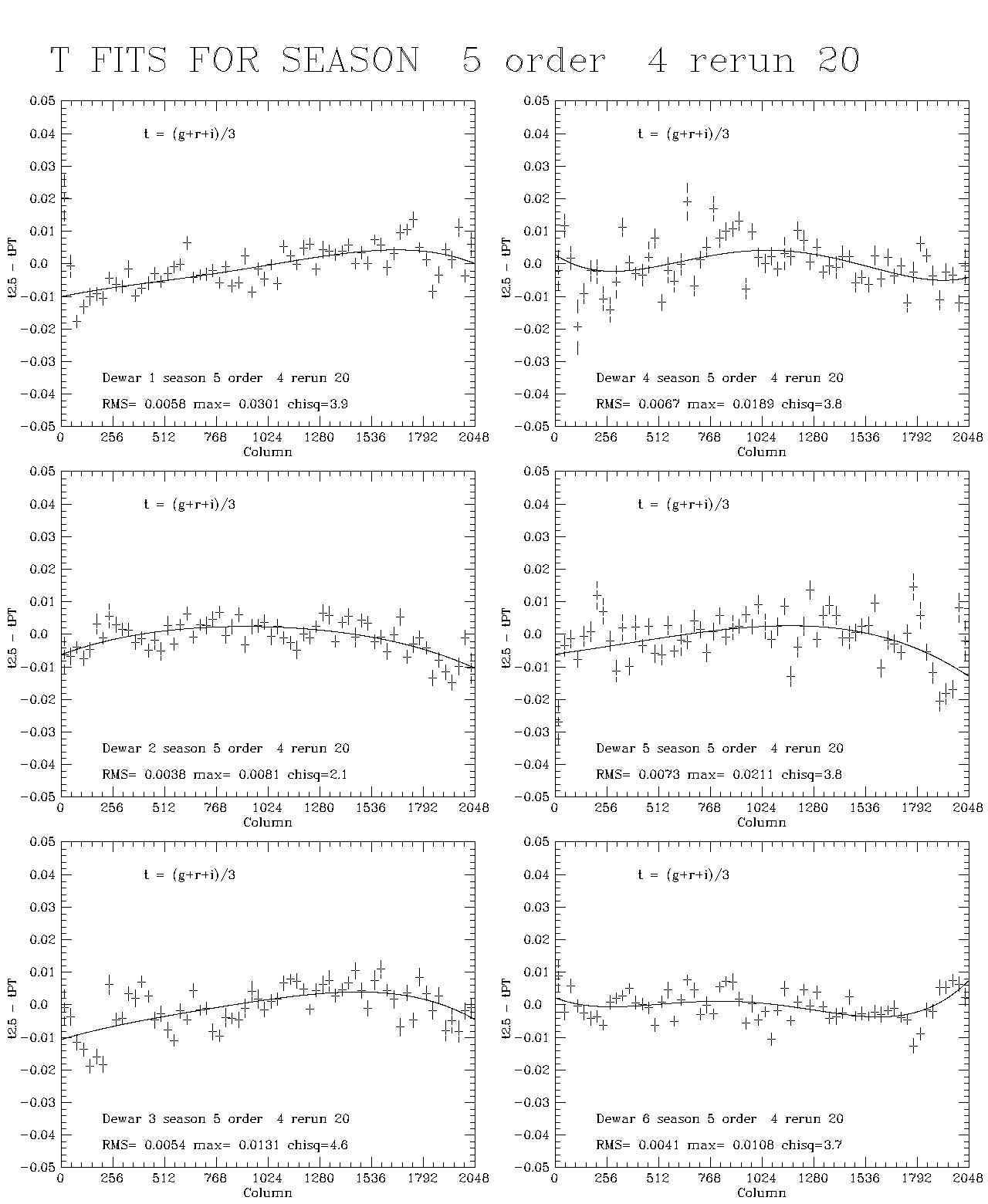
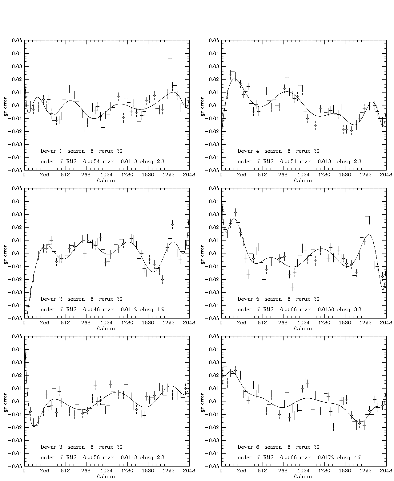
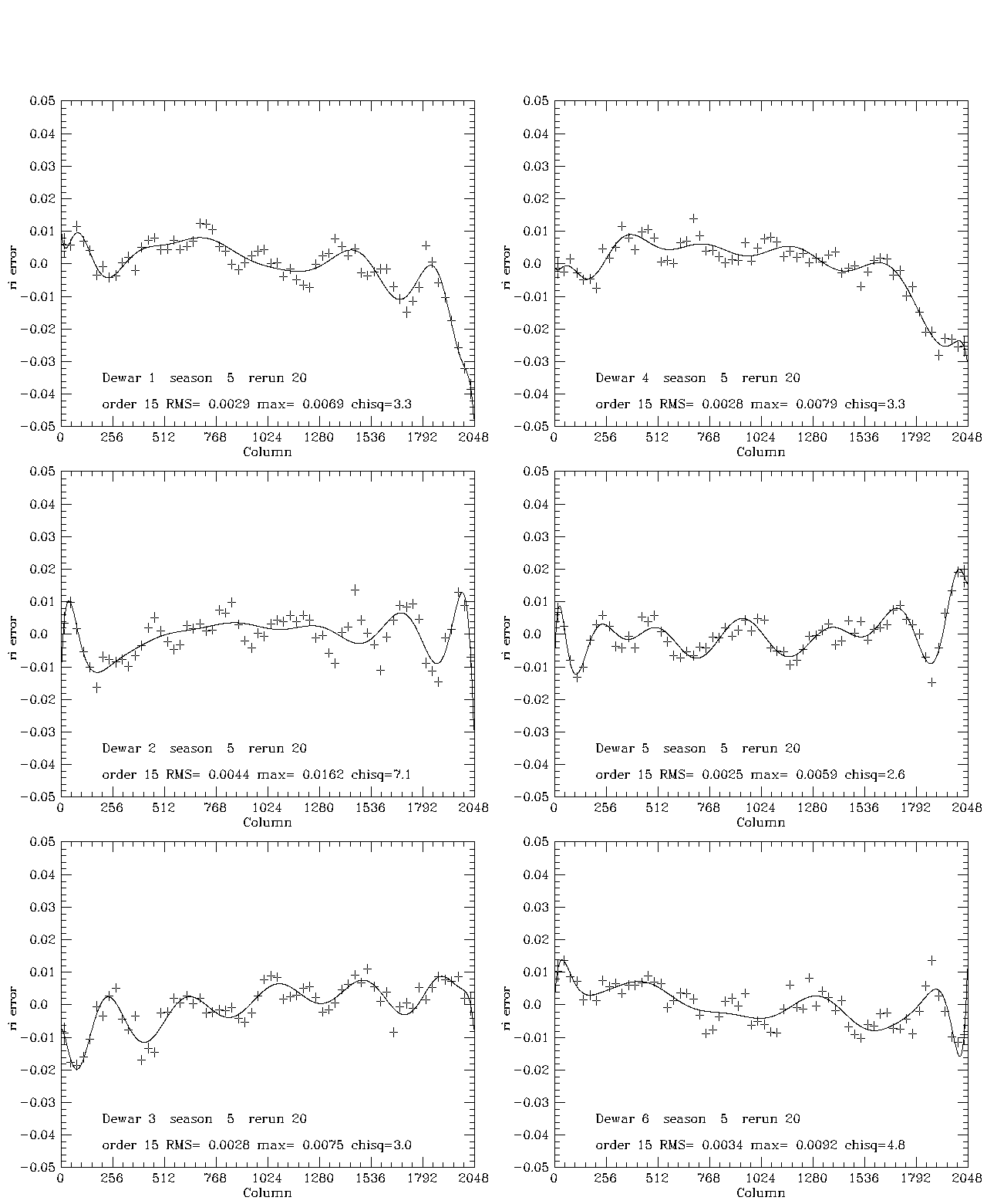
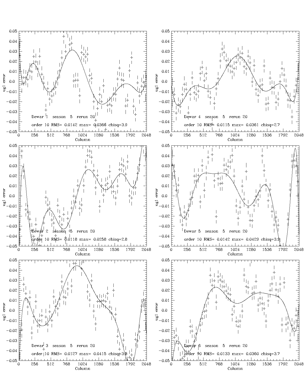
The bright cutoff is r = 15.0; only objects likely to be stars (|r_psf - r_model| < 0.2) are used and only those with good psfs (PSP_STATUS is OK), not BRIGHT, and not SATUR. All magnitudes are dereddened, which does not really matter on these scales. We thus begin with an initial guess about the flat fields (the `trial flats'), which can be the ones for the previous season, the ones derived from the sky medians, etc., run PHOTO, and use the derived photometry on the sets of objects defined by the photometry and the above definitions. If one averages over a group of camera columns, 32 in our case, each of these quantities has an average value (arranged to be near zero for the `perp' colors by appropriate choice of the constants in the above expressions) and a standard deviation which is the root sum square of the width of the stellar locus and the measuring errors. The locus width is typically 0.05 magnitudes in uperp1, uperp2, and g-r, and 0.03 magnitude in the others. The mean color is calculated using weights derived from these errors. If the flat field is correct, these colors will all be equal; if not, they will vary across the device. From these, one can algebraically derive the offsets which must be added to each of ug, gr, ri, and iz to achieve the best constancy across the device. The median offset for each of ug, gr, ri, and iz is arbitrarily set to zero; note that we are NOT setting photometric zero points, only variations in response across the device. So for each run/season (and typically the data for a single run do not define the flats well enough, and a large fraction of a whole season must be combined to do this) we produce a set of 64 points (bins of 32 columns across the 2048 columns of the CCD) of errors in the ratios of the flats--the gr error, for example, is delta_gr = -2.5*log((trueflat_g*trialflat_r)/(trialflat_g*trueflat_r)) These data are very powerful diagnostics, but do not give us enough to reconstruct the true flats, because there is only COLOR data, no magnitude data---in other words, we only have ratios in different colors of the ratios of the true flats to the trial ones. In practice, the errors in these 32-column bins are such that one is forced to do some smoothing to reduce the errors satisfactorily and reject points with large errors (typically caused by having too few stars in a bin, which unfortunately is usually at the ends where the scans do not overlap perfectly.) This was done by fitting a properly weighted Tchebychev polynomial to the values, of order chosen in each case to yield a satisfactory chi-squared. The orders are typically 10 to 15. III. Flattening the Flux Response Using the PTIn order to tie down the overall sensitivity, one must use something which determines the total flux sensitivity. One could use a well-measured color such as r from the PT for the calibration patches which both telescopes observe, and determine an r flat field from the photometric matches. If one does this, the full effect of flatfield errors in the PT, which are not well understood, enter the calibration of the 2.5-meter. If one has ONE such flat field and the color errors derived above, clearly, one can determine the corrections for all the devices in a camera column. We have chosen instead of doing this to at least average over what we hope are independent flat-field errors in the PT, by constructing a mean total magnitudet = (g + r + i)/3 We do not use z and u because they are typically less well measured and are known to have serious flatfielding problems in the PT; we do not know of serious errors in g, r, and i, and indeed tests involving measurements of a field on a grid of pointings suggest that the flats in these primary bands are determined to of order one percent. The procedure for using the t measurements is straightforward. In each of the 32-column wide bins, the measurements of the magnitude of each star in g, r, and i are compared between the PT and the 2.5-meter. It is assumed that the photometric error in the 2.5-meter is negligible and that the flat field is constant over the bin. Thus the scatter in the differences are measures of the PT measurement errors. These are determined in magnitude bins, and weights derived from these. For each bin, those weights are used to compute a mean difference and a chisquared, and stars are rejected if the difference from the mean is larger than 3 of the standard deviations appropriate for that star. These means and the associated standard deviations are then used to construct a set of difference values for t and associated errors. Again the median of the values for all the bins on a given device is subtracted - again we are not interested in photometric calibration, only in response differences at different places on the chip. It is somewhat disturbing that the chi-squared values for these differences are seldom as small as they should be, suggesting perhaps that there are problems at much higher spatial frequencies than we are resolving, but there is very little structure in the sky quartiles on these scales, so there is left something of a mystery. Given, then, these t difference values for each bin of columns, one can trivially derive the per-band flat-field errors: g = t + 2*gr/3 + ri/3, r = t - gr/3 + ri/3 i = t - gr/3 - 2*ri/3 z = i - iz u = g + ug Thus we derive a correction in each 32-column bin for each device in the camera. If the corrections are large enough (i.e. they affect the colors enough) that the data rejection in the determinations of the `perp' and ug colors used to derive the color corrections are significantly impacted, one must iterate again. This was not deemed necessary for DR1, and comparison of the predicted results for the first iterate and the measured one after the correction had been applied to the flats indicates in all cases that one iteration was sufficient for this data. These values in bins of 32 columns are again smoothed with weighted Tchebychev polynomials, here of order 4 because of the noisier data from the PT. The polynomial values as a function of column for the colors and t are then combined using the above relations to produce a set of corrections for each column of each device, and the new flat fields are then constructed by the application of those corrections. IV. Does it Work?The technique removes all of the low spatial frequency structure in the flat fields. It is unclear how much of the remaining rapid variations are real, but since (a) the sky quartiles do not show high spatial frequency structure, (b) we do not completely understand the statistics within the binned column data, and (c) the rapid, small amplitude variations which remain do not appear to be correlated from season to season, we suspect that they are just noise, though they are formally quite significant. Their nature and existence will become clear, we are sure, when oblique scan data are properly analyzed.
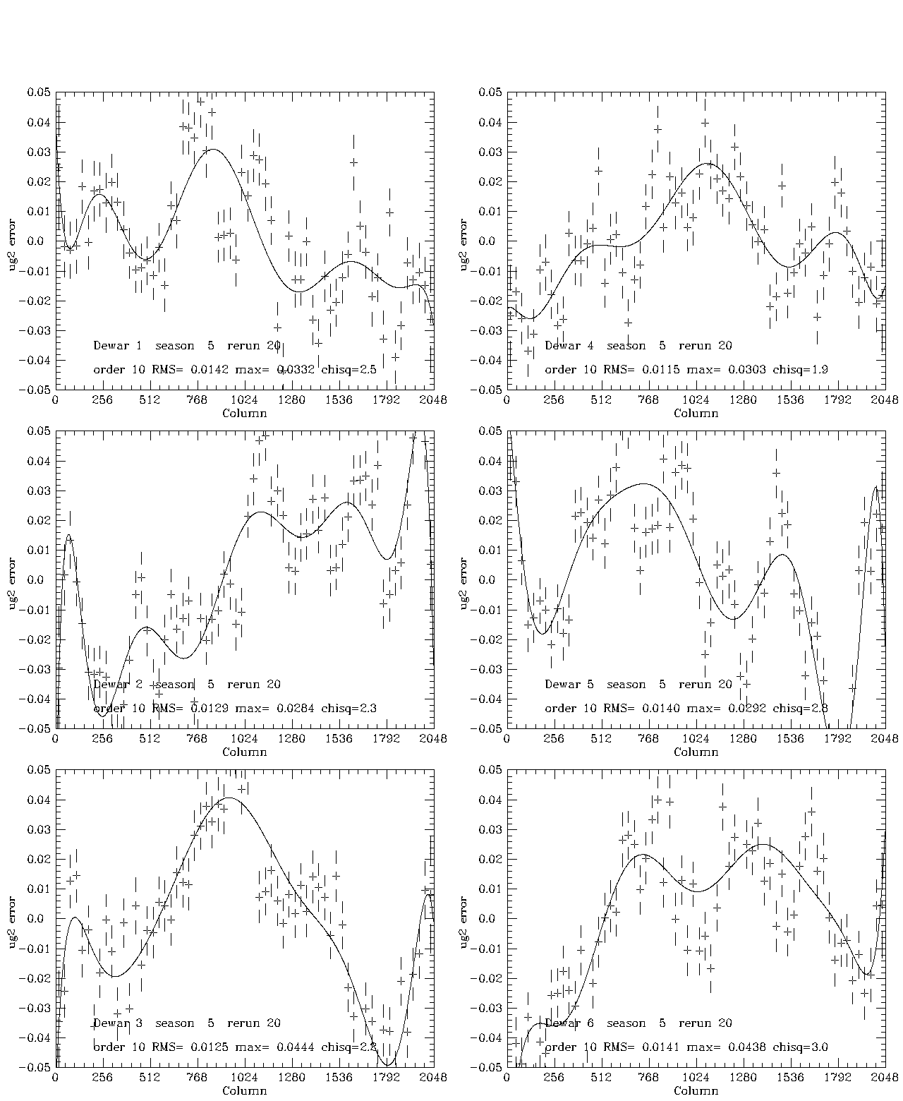
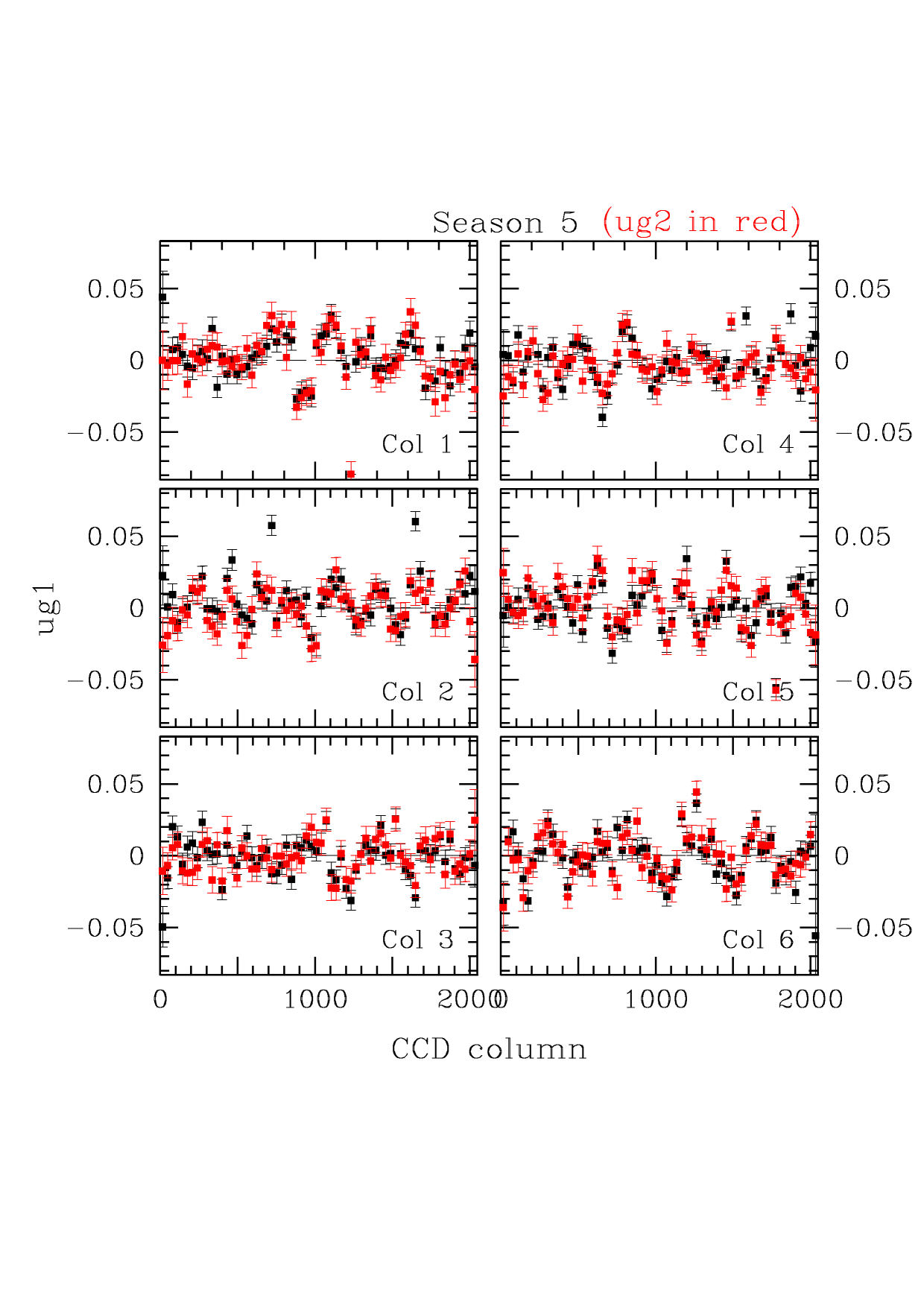
Five plots which illustrate the effect of the processing described are shown here for season 5, which was the least well-behaved season in this data set. Figure 1 illustrates the t fits for this season. The formal chi-squares/dof are large, of order 3-4, but the rms scatter about the fourth-order Tchebychev fit is of order 5-7 millimagnitudes. In most cases the polynomial is a very much better fit than a constant. The next four plots illustrate the fit to the color errors: gr (Fig. 2), ri(Fig. 3), ug1 (Fig. 4), and ug2 (Fig. 5). The two ug plots are shown to illustrate the excellent agreement between the two estimates, which are derived from uperp1 and uperp2, respectively. In these cases, the chi-squares are of the same order, and the rms deviations from the fits about 6, 3, 13, and 13 millimag, respectively. Since the ug1 and ug2 fits are averaged, the rms is about 10 millimag for ug and considerably smaller for the other bands. The color error dominates in u, the errors in t for all the other bands. Formally at least, the rms errors in the 5 bands are of order 12, 7, 6, 6, and 8 millimagnitudes for u, g, r, i, and z, respectively (the error in iz, not shown, is about 4 millimag). This is a sizeable part of the error budget for our goal of .02 magnitude RMS total, but since most of the rms is in small scale features whose reality is in doubt and we do not understand the noise very well, we may well be doing considerably better. We are at least doing no worse than these numbers, which ascribe no noise to the data. If one chooses to believe the chi-squares, the contribution of noise is only of order 10 percent of the error, but it may well, in fact, be most of it. The last plot, Figure 6, shows the ug color errors for the corrected data. This merely demonstrates that we did the arithmetic right and that, in fact, one iteration was sufficient in the worst band. Last modified: Mar 8 2004 |